5.1 Workflow

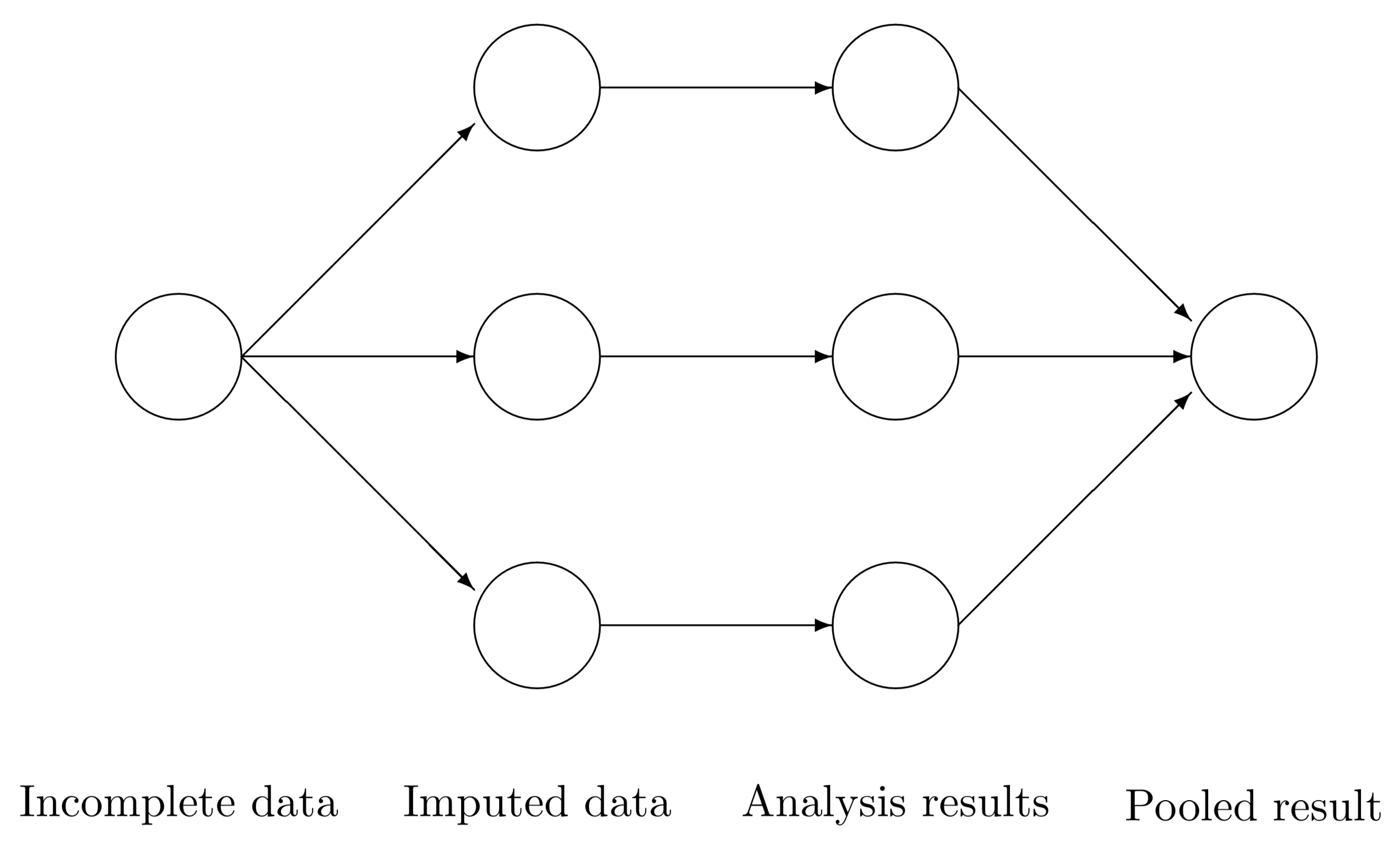
Figure 5.1: Scheme of main steps in multiple imputation.

Figure 5.1 outlines the three main steps in any multiple imputation analysis. In step 1, we create several $m$ complete versions of the data by replacing the missing values by plausible data values. The task of step 2 is to estimate the parameters of scientific or commercial interest from each imputed dataset. Step 3 involves pooling the $m$ parameter estimates into one estimate, and obtaining an estimate of its variance. The results allow us to arrive at valid decisions from the data, accounting for the missing data and having the correct type I error rate.

Table 5.1: Overview of the classes in the `mice` package.
Class	Name	Produced by	Description
`mids`	`imp`	`mice()`	multiply imputed dataset
`mild`	`idl`	`complete()`	multiply imputed list of data
`mira`	`fit`	`with()`	multiple imputation repeated analyses
`mipo`	`est`	`pool()`	multiple imputation pooled results

5.1.1 Recommended workflows

There is more than one way to divide the work that implements the steps of Figure 5.1. The classic workflow in mice runs functions mice(), with() and pool() in succession, each time saving the intermediate result:

# mids workflow using saved objects
library(mice)
imp <- mice(nhanes, seed = 123, print = FALSE)
fit <- with(imp, lm(chl ~ age + bmi + hyp))
est1 <- pool(fit)

The objects imp, fit and est have classes mids, mira and mipo, respectively. See Table 5.1 for an overview. The classic workflow works because mice contains a with() function that understands how to deal with a mids-object. The classic mids workflow has been widely adopted, but there are more possibilities.

The magrittr package introduced the pipe operator to R. This operator removes the need to save and reread objects, resulting in more compact and better readable code:

# mids workflow using pipes
library(magrittr)
est2 <- nhanes %>%
  mice(seed = 123, print = FALSE) %>%
  with(lm(chl ~ age + bmi + hyp)) %>%
  pool()

The with() function handles two tasks: to fill in the missing data and to analyze the data. Splitting these over two separate functions provided the user easier access to the imputed data, and hence is more flexible. The following code uses the complete() function to save the imputed data as a list of dataset (i.e., as an object with class mild), and then executes the analysis on each dataset by the lapply() function.

# mild workflow using base::lapply
est3 <- nhanes %>%
  mice(seed = 123, print = FALSE) %>%
  mice::complete("all") %>%
  lapply(lm, formula = chl ~ age + bmi + hyp) %>%
  pool()

If desired, we may extend the mild workflow by recycling through multiple arguments by means of the Map function.

# mild workflow using pipes and base::Map
est4 <- nhanes %>%
  mice(seed = 123, print = FALSE) %>%
  mice::complete("all") %>%
  Map(f = lm, MoreArgs = list(f = chl ~ age + bmi + hyp)) %>%
  pool()

RStudio has been highly successful with the introduction of the free and open tidyverse ecosystem for data acquisition, organization, analysis, visualization and reproducible research. The book by Wickham and Grolemund (2017) provides an excellent introduction to data science using tidyverse. The mild workflow can be written in tidyverse as

# mild workflow using purrr::map
library(purrr)
est5 <- nhanes %>%
  mice(seed = 123, print = FALSE) %>%
  mice::complete("all") %>%
  map(lm, formula = chl ~ age + bmi + hyp) %>%
  pool()

Manipulating the imputed data is easy if we store the imputed data in long format.

# long workflow using base::by
est6 <- nhanes %>%
  mice(seed = 123, print = FALSE) %>%
  mice::complete("long")  %>%
  by(as.factor(.$.imp), lm, formula = chl ~ age + bmi + hyp) %>%
  pool()

The long format can be processed by the dplyr::do() function into a list-column and pooled, as follows:

# long workflow using a dplyr list-column
library(dplyr)
est7 <- nhanes %>%
  mice(seed = 123, print = FALSE) %>%
  mice::complete("long") %>%
  group_by(.imp) %>%
  do(model = lm(formula = chl ~ age + bmi + hyp, data = .)) %>%
  as.list() %>%
  .[[-1]] %>%
  pool()

These workflows yield identical estimates, but allow for different extensions.

5.1.2 Not recommended workflow: Averaging the data

Researchers are often tempted to average the multiply imputed data, and analyze the averaged data as if it were complete. This method yields incorrect standard errors, confidence intervals and $p$-values, and thus should not be used if any form of statistical testing or uncertainty analysis is to be done on the imputed data. The reason is that the procedure ignores the between-imputation variability, and hence shares all the drawbacks of single imputation. See Section 1.3.

Averaging the data and analyzing the aggregate is easy to do with dplyr:

# incorrect workflow: averaging data, no pooling
ave <- nhanes %>%
  mice(seed = 123, print = FALSE) %>%
  mice::complete("long") %>%
  group_by(.id) %>%
  summarise_all(.funs = mean) %>%
  select(-.id, -.imp)
est8 <- lm(formula = chl ~ age + bmi + hyp, data = ave)

This workflow is faster and easier than the methods in Section 5.1.1, since there is no need to replicate the analyses $m$ times. In the words of Dempster and Rubin (1983), this workflow is

… seductive because it can lull the user into the pleasurable state of believing that the data are complete after all.

The ensuing statistical analysis does not know which data are observed and which are missing, and treats all data values as real, which will underestimate the uncertainty of the parameters. The reported standard errors and $p$-values after data-averaging are generally too low. The correlations between the variables of the averaged data will be too high. For example, the correlation matrix is the average data

cor(ave)

       age     bmi    hyp   chl
age  1.000 -0.4079 0.5262 0.478
bmi -0.408  1.0000 0.0308 0.313
hyp  0.526  0.0308 1.0000 0.381
chl  0.478  0.3127 0.3812 1.000

are more extreme than the average of the $m$ correlation matrices[^1]

cor <- nhanes %>%
  mice(seed = 123, print = FALSE) %>%
  mice::complete("all") %>%
  lapply(cor)
Reduce("+", cor) / length(cor)

       age     bmi    hyp   chl
age  1.000 -0.3676 0.4741 0.442
bmi -0.368  1.0000 0.0377 0.278
hyp  0.474  0.0377 1.0000 0.299
chl  0.442  0.2782 0.2985 1.000

which is an example of ecological fallacy. As researchers tend to like low $p$-values and high correlations, there is a cynical reward for the analysis of the average data. However, analysis of the average data cannot give a fair representation of the uncertainties associated with the underlying data, and hence is not recommended.

5.1.3 Not recommended workflow: Stack imputed data

A variation on this theme is to stack the imputed data, thus creating $m\times n$ complete records. Each record is weighted by a factor $1/m$, so that the total sample size is equal to $n$. The statistical analysis amounts to performing a weighted linear regression. If the scientific interest is restricted to point estimates and if the complete-data model is linear, this analysis of the stacked imputed data will yield unbiased estimates. Be aware that routine methods for calculating test statistics, confidence intervals or $p$-values will provide invalid answers if applied to the stacked imputed data.

Creating and analyzing a stacked imputed dataset is easy:

est9 <- nhanes2 %>%
  mice(seed = 123, print = FALSE) %>%
  mice::complete("long") %>%
  lm(formula = chl ~ age + bmi + hyp)

While the estimated regression coefficients are unbiased, we cannot trust the standard errors, $t$-values and so on. An advantage of stacking over averaging is that it is easier to analyze categorical data. Although stacking can be useful in specific contexts, like variable selection, in general it is not recommended.

5.1.4 Repeated analyses

The appropriate way to analyze multiply imputed data is to fit the complete-data model on each imputed dataset separately. In mice we can use the with() command for this purpose. This function takes two main arguments. The first argument of the call is a mids object produced by mice(). The second argument is an expression that is to be applied to each completed dataset. The with() function implements the following loop ($\ell=1,\dots,m$):

it creates the $\ell^\mathrm{th}$ imputed dataset
it runs the expression on the imputed dataset
it stores the result in the list fit$analyses

For example, we fit a regression model to each dataset and print out the estimates from the first and second completed datasets by

fit <- with(imp, lm(chl~bmi+age))
coef(fit$analyses[[1]])

(Intercept)         bmi         age 
      33.55        4.08       27.37

coef(fit$analyses[[2]])

(Intercept)         bmi         age 
     -51.47        6.77       35.44

Note that the estimates differ from each other because of the uncertainty created by the missing data. Applying the standard pooling rules is done by

est <- pool(fit)
summary(est)

            estimate std.error statistic    df p.value
(Intercept)     6.26     64.29    0.0974  9.62 0.92394
bmi             4.99      2.10    2.3762  9.24 0.03370
age            29.17      9.15    3.1890 12.89 0.00718

which shows the correct estimates after multiple imputation.

Any R expression produced by expression() can be evaluated on the multiply imputed data. For example, suppose we want to calculate the difference in frequencies between categories 1 and 2 of hyp. This is conveniently done by the following statements:

expr <- expression(freq <- table(hyp), freq[1] - freq[2])
fit <- with(imp, eval(expr))
unlist(fit$analyses)

 1  1  1  1  1 
 9  9 11 15 15

All the major software packages nowadays have ways to execute the $m$ repeated analyses to the imputed data.