9.1 Too many columns

Suppose that your colleague has become enthusiastic about multiple imputation. She asked you to create a multiply imputed version of her data, and forwarded you her entire database. As a first step, you use R to read it into a data frame called data. After this is done, you type in the following commands:

library(mice)
## DO NOT DO THIS
imp <- mice(data)     # not recommended

If you are lucky, the program may run and impute, but after a few minutes it becomes clear that it takes a long time to finish. And after the wait is over, the imputations turn out to be surprisingly bad. What happened?

Some exploration of the data reveals that your colleague sent you a dataset with 351 columns, essentially all the information that was sampled in the study. By default, the mice() function uses all other variables as predictors, so mice() will try to calculate regression analyses with 350 explanatory variables, and repeat that for every incomplete variable. Categorical variables are internally represented as dummy variables, so the actual number of predictors could easily double. This makes the algorithm extremely slow, if it runs at all.

Some further exploration reveals some variables are free text fields, and that some of the missing values were not marked as such in the data. As a consequence, mice() treats impossible values such as “999” or “-1” as real data. Just one forgotten missing data mark may introduce large errors into the imputations.

In order to evade such practical issues, it is necessary to spend some time exploring the data first. Furthermore, it is helpful if you understand for which scientific question the data are used. Both will help in creating sensible imputations.

This section concentrates on what can be done based on the data values themselves. In practice, it is far more productive and preferable to work together with someone who knows the data really well, and who knows the questions of scientific interest that one could ask from the data. Sometimes the possibilities for cooperation are limited. This may occur, for example, if the data have come from several external sources (as in meta analysis), or if the dataset is so diverse that no one person can cover all of its contents. It will be clear that this situation calls for a careful assessment of the data quality, well before attempting imputation.

9.1.1 Scientific question

There is a paradoxical inverse relation between blood pressure (BP) and mortality in persons over 85 years of age (Boshuizen et al. 1998; Van Bemmel et al. 2006). Normally, people with a lower BP live longer, but the oldest old with lower BP live a shorter time.

The goal of the study was to determine if the relation between BP and mortality in the very old is due to frailty. A second goal was to know whether high BP was a still risk factor for mortality after the effects of poor health had been taken into account.

The study compared two models:

1. The relation between mortality and BP adjusted for age, sex and type of residence.

2. The relation between mortality and BP adjusted for age, sex, type of residence and health.

Health was measured by 28 different variables, including mental state, handicaps, being dependent in activities of daily living, history of cancer and others. Including health as a set of covariates in model 2 might explain the relation between mortality and BP, which, in turn, has implications for the treatment of hypertension in the very old.

9.1.2 Leiden 85+ Cohort

The data come from the 1236 citizens of Leiden who were 85 years or older on December 1, 1986 (Lagaay, Van der Meij, and Hijmans 1992; Izaks et al. 1997). These individuals were visited by a physician between January 1987 and May 1989. A full medical history, information on current use of drugs, a venous blood sample, and other health-related data were obtained. BP was routinely measured during the visit. Apart from some individuals who were bedridden, BP was measured while seated. An Hg manometer was used and BP was rounded to the nearest 5 mmHg. Measurements were usually taken near the end of the interview. The mortality status of each individual on March 1, 1994 was retrieved from administrative sources.

Of the original cohort, a total of 218 persons died before they could be visited, 59 persons did not want to participate (some because of health problems), 2 emigrated and 1 was erroneously not interviewed, so 956 individuals were visited. Effects due to subsampling the visited persons from the entire cohort were taken into account by defining the date of the home visit as the start (Boshuizen et al. 1998). This type of selection will not be considered further.

9.1.3 Data exploration

The data are stored as a SAS export file. The read.xport() function from the foreign package can read the data.

library(foreign)
file.sas <- "data/c85/master85.xport"
original.sas <- read.xport(file.sas)
names(original.sas) <- tolower(names(original.sas))
dim(original.sas)

[1] 1236  351

The dataset contains 1236 rows and 351 columns. When I tracked down the origin of the data, the former investigators informed me that the file was composed during the early 1990’s from several parts. The basic component consisted of a Dbase file with many free text fields. A dedicated Fortran program was used to separate free text fields. All fields with medical and drug-related information were hand-checked against the original forms. The information not needed for analysis was not cleaned. All information was kept, so the file contains several versions of the same variable.

A first scan of the data makes clear that some variables are free text fields, person codes and so on. Since these fields cannot be sensibly imputed, they are removed from the data. In addition, only the 956 cases that were initially visited are selected, as follows:

# remove 15 columns (text, administrative)
all <- names(original.sas)
drop <- c(3, 22, 58, 162:170, 206:208)
keep <- !(1:length(all) %in% drop)
leiden85 <- original.sas[original.sas$abr == "1", keep]
data <- leiden85

The frequency distribution of the missing cases per variable can be obtained as:

ini <- mice(data, maxit = 0)   # recommended

Warning: Number of logged events: 28

table(ini$nmis)

  0   2   3   5   7  14  15  28  29  32  33  34  35  36  40  42 
 87   2   1   1   1   1   2   1   3   2  34  15  25   4   1   1 
 43  44  45  46  47  48  49  50  51  54  64  72  85 103 121 126 
  2   1   4   2   3  24   4   1  20   2   1   4   1   1   1   1 
137 155 157 168 169 201 202 228 229 230 231 232 233 238 333 350 
  1   1   1   2   1   7   3   5   4   2   4   1   1   1   3   1 
501 606 635 636 639 642 722 752 753 812 827 831 880 891 911 913 
  3   1   2   1   1   2   1   5   3   1   1   3   3   3   3   1 
919 928 953 954 955 
  1   1   3   3   3 

Ignoring the warning for a moment, we see that there are 87 variables that are complete. The set includes administrative variables (e.g., person number), design factors, date of measurement, survival indicators, selection variables and so on. The set also included some variables for which the missing data were inadvertently not marked, containing values such as “999” or “-1.” For example, the frequency distribution of the complete variable “beroep1” (occupation) is

table(data$beroep1, useNA = "always")

  -1    0    1    2    3    4    5    6 <NA> 
  42    1  576  125  104   47   44   17    0 

There are no missing values, but a variable with just categories “-1” and “0” is suspect. The category “-1” likely indicates that the information was missing (this was the case indeed). One option is to leave this “as is,” so that mice() treats it as complete information. All cases with a missing occupation are then seen as a homogeneous group.

Two other variables without missing data markers are syst and diast, i.e., systolic and diastolic BP classified into six groups. The correlation (using the observed pairs) between syst and rrsyst, the variable of primary interest, is 0.97. Including syst into the imputation model for rrsyst will ruin the imputations. The “as is” option is dangerous, and shares some of the same perils of the indicator method (cf. Section 1.3.7). The message is that variables that are 100% complete deserve appropriate attention.

After a first round of screening, I found that 57 of the 87 complete variables were uninteresting or problematic in some sense. Their names were placed on a list named outlist1 as follows:

v1 <- names(ini$nmis[ini$nmis == 0])
outlist1 <- v1[c(1, 3:5, 7:10, 16:47, 51:60, 62, 64:65, 69:72)]
length(outlist1)

[1] 57

9.1.4 Outflux

We should also scrutinize the variables at the other end. Variables with high proportions of missing data generally create more problems than they solve. Unless some of these variables are of genuine interest to the investigator, it is best to leave them out. Virtually every dataset contains some parts that could better be removed before imputation. This includes, but is not limited to, uninteresting variables with a high proportion of missing data, variables without a code for the missing data, administrative variables, constant variables, duplicated, recoded or standardized variables, and aggregates and indices of other information.

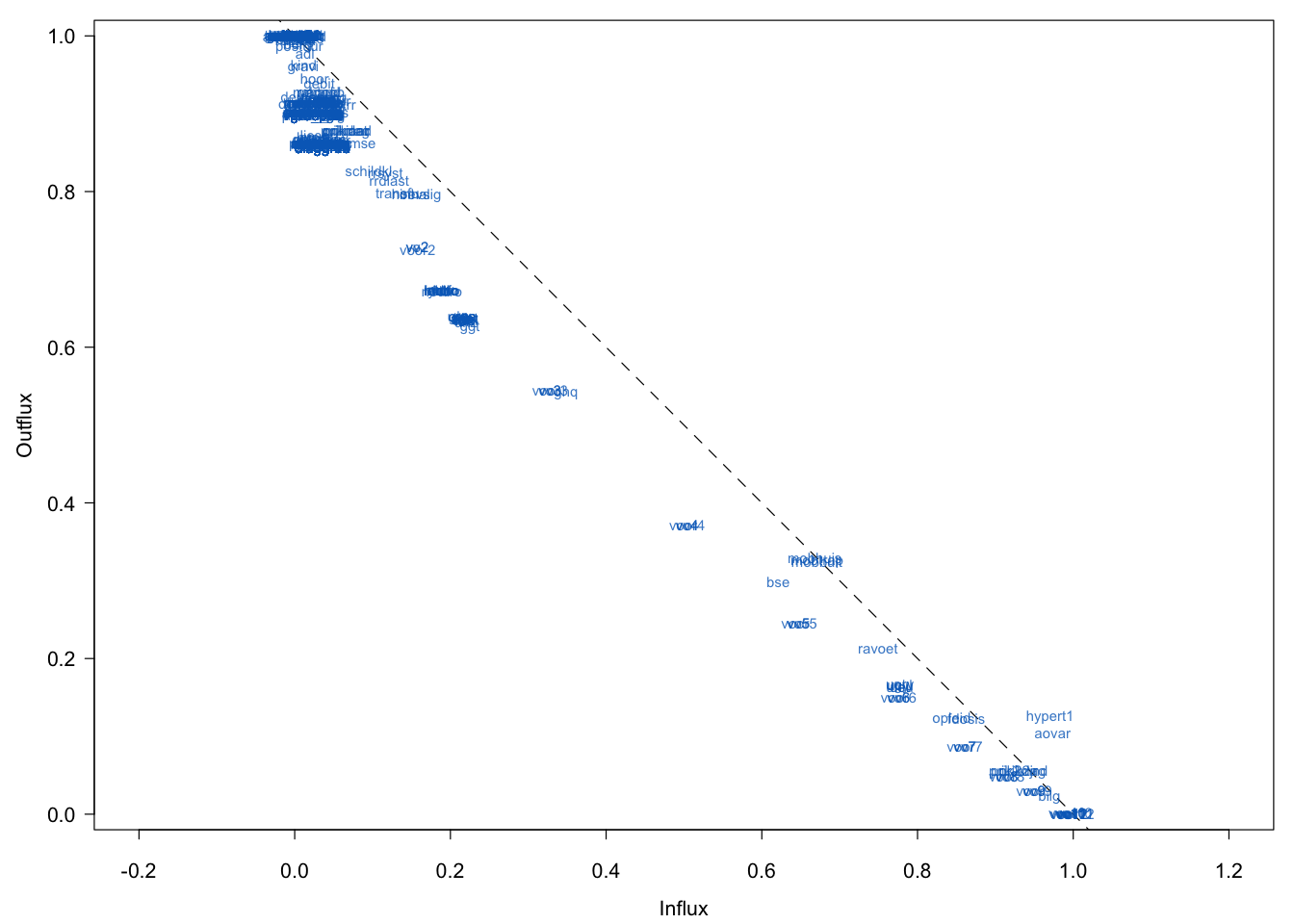
Figure 9.1: Global influx-outflux pattern of the Leiden 85+ Cohort data. Variables with higher outflux are (potentially) the more powerful predictors. Variables with higher influx depend strongly on the imputation model.

Figure 9.1 is the influx-outflux pattern of Leiden 85+ Cohort data. The influx of a variable quantifies how well its missing data connect to the observed data on other variables. The outflux of a variable quantifies how well its observed data connect to the missing data on other variables. See Section 4.1.3 for more details. Though the display could obviously benefit from a better label-placing strategy, we can see three groups. All points are relatively close to the diagonal, which indicates that influx and outflux are balanced.

The group at the left-upper corner has (almost) complete information, so the number of missing data problems for this group is relatively small. The intermediate group has an outflux between 0.5 and 0.8, which is small. Missing data problems are more severe, but potentially this group could contain important variables. The third group has an outflux with 0.5 and lower, so its predictive power is limited. Also, this group has a high influx, and is thus highly dependent on the imputation model.

Note that there are two variables (hypert1 and aovar) in the third group that are located above the diagonal. Closer inspection reveals that the missing data mark had not been set for these two variables. Variables that might cause problems later on in the imputations are located in the lower-right corner. Under the assumption that this group does not contain variables of scientific interest, I transferred 45 variables with an outflux < 0.5 to outlist2:

outlist2 <- row.names(fx)[fx$outflux < 0.5]
length(outlist2)

[1] 45

In these data, the set of selected variables is identical to the group with more than 500 missing values, but this need not always be the case. I removed the 45 variables, recalculated influx and outflux on the smaller dataset and selected 32 new variables with outflux < 0.5.

data2 <- data[, !names(data) %in% outlist2]
fx2 <- flux(data2)
outlist3 <- row.names(fx2)[fx2$outflux < 0.5]

Variable outlist3 contains 32 variable names, among which are many laboratory measurements. I prefer to keep these for imputation since they may correlate well with BP and survival. Note that the outflux changed considerably as I removed the 45 least observed variables. Influx remained nearly the same.

9.1.5 Finding problems: loggedEvents

Another source of information is the list of logged events produced by mice(). The warning we ignored previously indicates that mice found some peculiarities in the data that need the user’s attention. The logged events form a structured report that identify problems with the data, and details which corrective actions were taken by mice(). It is a component called loggedEvents of the mids object.

head(ini$loggedEvents, 2)

  it im dep     meth out
1  0  0     constant abr
2  0  0     constant vo7

tail(ini$loggedEvents, 2)

   it im dep      meth    out
27  0  0     collinear voor10
28  0  0     collinear voor11

At initialization, a log entry is made for the following actions:

• A constant variable is removed from the imputation model, unless the remove.constant = FALSE argument is specified;

• A variable that is collinear with another variable is removed from the imputation model, unless the remove.collinear = FALSE argument is specified.

A variable is removed from the model by internal edits of the predictorMatrix, method, visitSequence and post components of the model. The data are kept intact. Note that setting remove.constant = FALSE or remove.collinear = FALSE bypasses usual safety measures in mice, and could cause problems further down the road. If a variable has only NA’s, it is considered a constant variable, and will not be imputed. Setting remove.constant = FALSE will cause numerical problems since there are no observed cases to estimate the imputation model, but such variables can be imputed by passive imputation by specifying the allow.na = TRUE argument.

During execution of the main algorithm, the entries in loggedEvents can signal the following actions:

• A predictor that is constant or correlates higher than 0.999 with the target variable is removed from the univariate imputation model. The cut-off value can be specified by the threshold argument;

• If all predictors are removed, this is noted in loggedEvents, and the imputation model becomes an intercept-only model;

• The degrees of freedom can become negative, usually because there are too many predictors relative to the number of observed values for the target. In that case, the degrees of freedom are set to 1, and a note is written to loggedEvents.

A few events may happen just by chance, in which case they are benign. However, if there are many entries, it is likely that the imputation model is overparametrized, causing sluggish behavior and unstable estimates. In that case, the imputation model needs to be simplified.

The loggedEvents component of the mids object is a data frame with five columns. The columns it, im stand for iteration and imputation number. The column dep contains the name of the target variable, and is left blank at initialization. Column meth entry signals the type of problem, e.g. constant, df set to 1, and so on. Finally, the column out contains the names of the removed variables. The loggedEvents component contains vital hints about possible problems with the imputation model. Closer examination of these logs could provide insight into the nature of the problem. In general, strive for zero entries, in which case the loggedEvent component is equal to NULL.

Unfortunately, loggedEvents is not available if mice crashes. If that happens, inspect the console output to see what the last variable was, and think of reasons that might have caused the breakdown, e.g., using a categorical predictor with many categories as a predictor. Then remove this from the model. Alternatively, lowering maxit, setting ridge to a high value (ridge = 0.01), or using a more robust imputation method (e.g., pmm) may get you beyond the point where the program broke down. Then, obtain loggedEvents to detect any problems.

Continuing with the analysis, based on the initial output by mice(), I placed the names of all constant and collinear variables on outlist4 by

outlist4 <- as.character(ini$loggedEvents[, "out"])

This outlist contains 28 variables.

9.1.6 Quick predictor selection: quickpred

The mice package contains the function quickpred() that implements the predictor selection strategy of Section 6.3.2. In order to apply this strategy to the Leiden 85+ Cohort data, I first deleted the variables on three of the four outlists created in the previous sections.

outlist <- unique(c(outlist1, outlist2, outlist4))
length(outlist)

[1] 108

There are 108 unique variables to be removed. Thus, before doing any imputations, I cleaned out about one third of the data that are likely to cause problems. The downsized data are

data2 <- data[, !names(data) %in% outlist]

The next step is to build the imputation model according to the strategy outlined above. The function quickpred() is applied as follows:

inlist <- c("sex", "lftanam", "rrsyst", "rrdiast")
pred <- quickpred(data2, minpuc = 0.5, include = inlist)

There are 198 incomplete variables in data2. The character vector inlist specifies the names of the variables that should be included as covariates in every imputation model. Here I specified age, sex and blood pressure. Blood pressure is the variable of central interest, so I included it in all models. This list could be longer if there are more outcome variables. The inlist could also include design factors.

The quickpred() function creates a binary predictor matrix of 198 rows and 198 columns. The rows correspond to the incomplete variables and the columns report the same variables in their role as predictor. The number of predictors varies per row. We can display the distribution of the number of predictors by

table(rowSums(pred))

 0  7 11 12 13 14 15 16 17 18 19 20 21 22 23 24 25 26 27 28 29 
30  1  2  1  1  2  5  2 13  8 16  9 13  7  5  6 10  6  3  6  4 
30 31 32 33 34 35 36 37 38 39 40 41 42 44 45 46 49 50 57 59 60 
 8  3  6  9  2  4  6  2  5  2  4  2  3  4  3  3  3  1  1  1  1 
61 68 79 83 85 
 1  1  1  1  1 

The variability in model sizes is substantial. The 30 rows with no predictors are complete. The mean number of predictors is equal to 24.8. It is possible to influence the number of predictors by altering the values of mincor and minpuc in quickpred(). A number of predictors of 15–25 is about right (cf. Section 6.3.2), so I decided to accept this predictor matrix. The number of predictors for systolic and diastolic BP are

rowSums(pred[c("rrsyst", "rrdiast"),])

 rrsyst rrdiast 
     41      36 

The names of the predictors for rrsyst can be obtained by

names(data2)[pred["rrsyst", ] == 1]

It is sometimes useful the inspect the correlations of the predictors selected by quickpred(). Table 3 in Van Buuren, Boshuizen, and Knook (1999) provides an example. For a given variable, the correlations can be tabulated by

vname <- "rrsyst"
y <- cbind(data2[vname], r =! is.na(data2[, vname]))
vdata <- data2[,pred[vname,] == 1]
round(cor(y = y, x = vdata, use = "pair"), 2)

9.1.7 Generating the imputations

Everything is now ready to impute the data as

imp.qp <- mice(data2, pred = pred, seed = 29725)

Thanks to the smaller dataset and the more compact imputation model, this code runs about 50 times faster than “blind imputation” as practiced in Section 9.1. More importantly, the new solution is much better. To illustrate the latter, take a look at Figure 9.2.

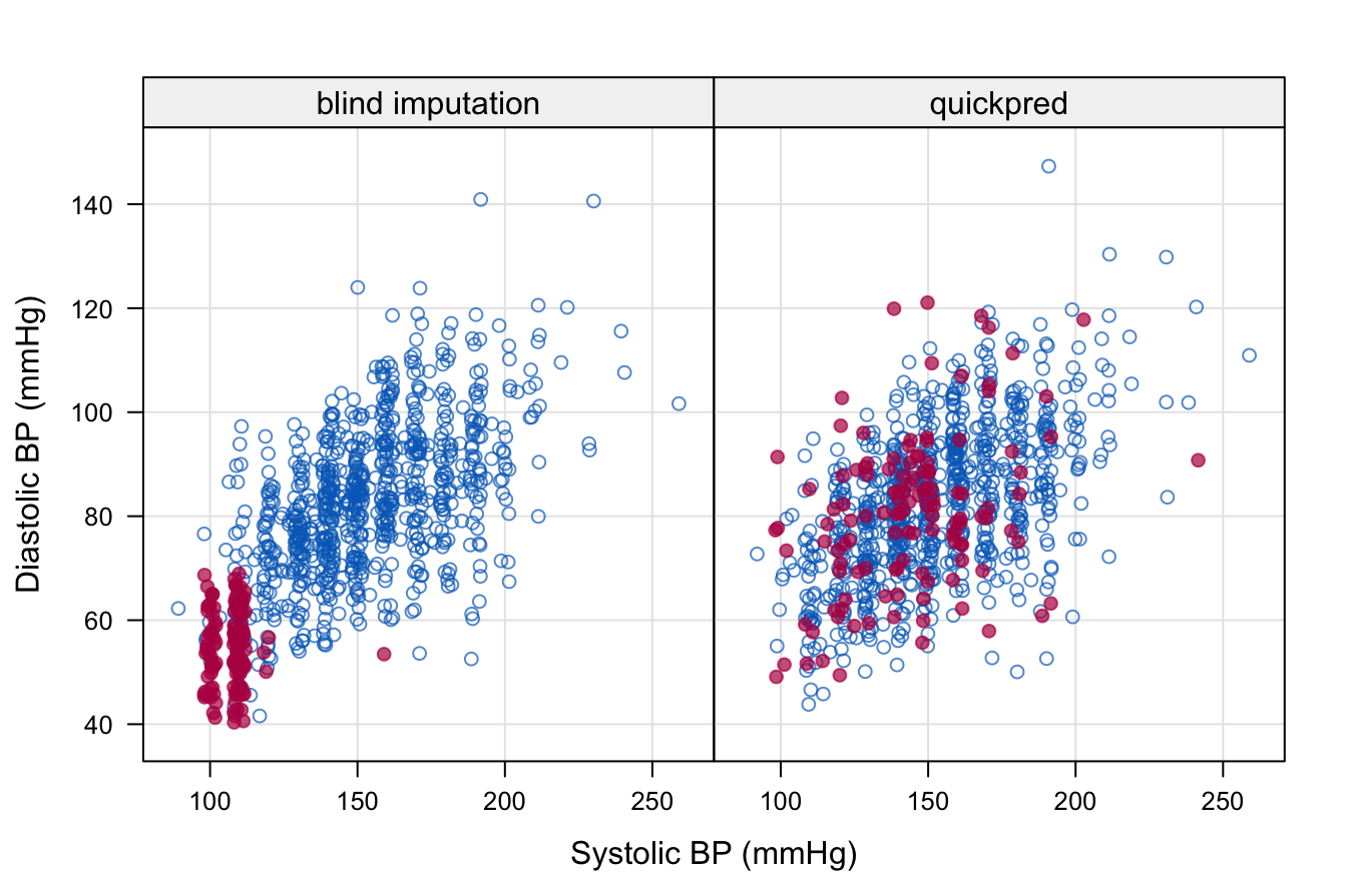
Figure 9.2: Scatterplot of systolic and diastolic blood pressure from the first imputation. The left-hand-side plot was obtained after just running mice() on the data without any data screening. The right-hand-side plot is the result after cleaning the data and setting up the predictor matrix with quickpred(). Leiden 85+ Cohort data.

The figure is the scatterplot of rrsyst and rrdiast of the first imputed dataset. The left-hand figure shows what can happen if the data are not properly screened. In this particular instance, a forgotten missing data mark of “-1” was counted as a valid blood pressure value, and produced imputation that are far off. In contrast, the imputations created with the help of quickpred() look reasonable.

The plot was created by the following code:

vnames <- c("rrsyst", "rrdiast")
cd1 <- mice::complete(imp)[, vnames]
cd2 <- mice::complete(imp.qp)[, vnames]
typ <- factor(rep(c("blind imputation", "quickpred"),
                  each = nrow(cd1)))
mis <- ici(data2[, vnames])
mis <- is.na(imp$data$rrsyst) | is.na(imp$data$rrdiast)
cd <- data.frame(typ = typ, mis = mis, rbind(cd1, cd2))
xyplot(jitter(rrdiast, 10) ~ jitter(rrsyst, 10) | typ,
       data = cd, groups = mis,
       col = c(mdc(1), mdc(2)),
       xlab = "Systolic BP (mmHg)",
       type = c("g","p"), ylab = "Diastolic BP (mmHg)",
       pch = c(1, 19),
       strip = strip.custom(bg = "grey95"),
       scales = list(alternating = 1, tck = c(1, 0)))

9.1.8 A further improvement: Survival as predictor variable

If the complete-data model is a survival model, incorporating the cumulative hazard to the survival time, \(H_0(T)\), as one of the predictors provide slightly better imputations (White and Royston 2009). In addition, the event indicator should be included into the model. The Nelson-Aalen estimate of \(H_0(T)\) in the Leiden 85+ Cohort can be calculated as

dat <- cbind(data2, dead = 1 - data2$dwa)
hazard <- nelsonaalen(dat, survda, dead)

where dead is coded such that “1” means death. The nelsonaalen() function is part of mice. Table 9.1 lists the correlations beween several key variables. The correlation between \(H_0(T)\) and \(T\) is almost equal to 1, so for these data it matters little whether we take \(H_0(T)\) or \(T\) as the predictor. The high correlation may be caused by the fact that nearly everyone in this cohort has died, so the percentage of censoring is low. The correlation between \(H_0(T)\) and \(T\) could be lower in other epidemiological studies, and thus it might matter whether we take \(H_0(T)\) or \(T\). Observe that the correlation between log(\(T\)) and blood pressure is higher than for \(H_0(T)\) or \(T\), so it makes sense to add log(\(T\)) as an additional predictor. This strong relation may have been a consequence of the design, as the frail people were measured first.

Table 9.1: Pearson correlations between the cumulative death hazard \(H_0(T)\), survival time \(T\), log(\(T\)), systolic and diastolic blood pressure.

	\(H_0(T)\)	\(T\)	log(\(T\))	SBP	DBP
\(H_0(T)\)	1.000	0.997	0.830	0.169	0.137
\(T\)	0.997	1.000	0.862	0.176	0.141
log(\(T\))	0.830	0.862	1.000	0.205	0.151
SBP	0.169	0.176	0.205	1.000	0.592
DBP	0.137	0.141	0.151	0.592	1.000

9.1.9 Some guidance

Imputing data with many columns is challenging. Even the most carefully designed and well-maintained data may contain information or errors that can send the imputations awry. I conclude this section by summarizing advice for imputation of data with “too many columns.”

1. Inspect all complete variables for forgotten missing data marks. Repair or remove these variables. Even one forgotten mark may ruin the imputation model. Remove outliers with improbable values.

2. Obtain insight into the strong and weak parts of the data by studying the influx-outflux pattern. Unless they are scientifically important, remove variables with low outflux, or with high fractions of missing data.

3. Perform a dry run with maxit=0 and inspect the logged events produced by mice(). Remove any constant and collinear variables before imputation.

4. Find out what will happen after the data have been imputed. Determine a set of variables that are important in subsequent analyses, and include these as predictors in all models. Transform variables to improve predictability and coherence in the complete-data model.

5. Run quickpred(), and determine values of mincor and minpuc such that the average number of predictors is around 25.

6. After imputation, determine whether the generated imputations are sensible by comparing them to the observed information, and to knowledge external to the data. Revise the model where needed.

7. Document your actions and decisions, and obtain feedback from the owner of the data.

It is most helpful to try out these techniques on data gathered within your own institute. Some of these steps may not be relevant for other data. Determine where you need to adapt the procedure to suit your needs.