7.7 Discrete outcome

This section details how to create multiple imputations under the multilevel model when missing values occur in a discrete outcome only.

7.7.1 Methods

The generalized linear mixed model (GLMM) extends the mixed model for continuous data with link functions. For example, we can draw imputations for clustered binary data by positing a logit link with a binomial distribution. As before, all parameters need to be drawn from their respective posteriors in order to account for the sampling variation.

Jolani et al. (2015) developed a multilevel imputation method for binary data obtaining estimates of the parameters of model by the lme4::glmer() function in lme4 package (Bates et al. 2015), followed by a sequence of random draws from the parameter distributions. For meta-analysis of individual participant data, this method outperforms simpler methods that ignore the clustering, that assume MCAR or that split the data by cluster (Jolani et al. 2015). The method is available as method 2l.bin in mice. The miceadds package Robitzsch, Grund, and Henke (2017) contains a method 2l.binary that allows the user to choose between likelihood estimation with lme4::glmer() and penalized ML with blme::bglmer() (Chung et al. 2013). Related methods are available under sequential hierarchical regression imputation (SHRIMP) framework (Yucel 2017).

Resche-Rigon and White (2018) proposed a two-stage estimator. At step 1, a linear regression model is fitted to each observed cluster. Any sporadically missing data are imputed, and the model per cluster ignores any systematically missing variables. At step 2, estimates obtained from each cluster are combined using meta-analysis. Systematically missing variables are modeled through a linear random effect model across clusters. A method for binary data is available as the method 2l.2stage.bin in the micemd package. The two-stage estimator is related to work done by Gelman, King, and Liu (1998) on data combinations of different surveys. These authors fitted a separate imputation for each survey using only the questions posed in the survey, and used hierarchical meta-analysis to combine the results from different surveys. Their term “not asked” translates into “systematically missing”, whereas “not answered” translates into “sporadically missing”.

Missing level-1 count outcomes can be imputed under the generalized linear mixed model using a Poisson or (zero-inflated) negative binomial distributions (Kleinke and Reinecke 2015). Relevant functions can be found in the micemd and countimp packages. Table 7.3 presents an overview of R functions for univariate imputations for discrete outcomes. Discrete data can also be imputed by the predictive mean matching functions listed in Table 7.2.

Table 7.3: Methods to perform univariate multilevel imputation of missing discrete outcomes. Each of the methods is available as a function called mice.impute.[method] in the specified R package.

Package	Method	Description
Binary
mice	2l.bin	logistic, glmer
miceadds	2l.binary	logistic, glmer
micemd	2l.2stage.bin	logistic, mvmeta
micemd	2l.glm.bin	logistic, glmer
Count
micemd	2l.2stage.pois	Poisson, mvmeta
micemd	2l.glm.pois	Poisson, glmer
countimp	2l.poisson	Poisson, glmmPQL
countimp	2l.nb2	negative binomial, glmmadmb
countimp	2l.zihnb	zero-infl neg bin, glmmadmb

7.7.2 Example

The toenail data were collected in a randomized parallel group trial comparing two treatments for a common toenail infection. A total of 294 patients were seen at seven visits, and severity of infection was dichotomized as “not severe” (0) and “severe” (1). The version of the data in the DPpackage is all numeric and easy to analyze. The following statements load the data, and expand the data to the full design with \(7 \times 294 = 2058\) rows. There are in total 150 missed visits.

library(tidyr)
data("toenail", package = "DPpackage")
data <- tidyr::complete(toenail, ID, visit) %>%
  tidyr::fill(treatment) %>%
  dplyr::select(-month)
table(data$outcome, useNA = "always")

   0    1 <NA> 
1500  408  150 

Molenberghs and Verbeke (2005) described various analyses of these data. Here we impute the outcome of the missed visits. The next code block declares ID as the cluster variable, and creates \(m=5\) imputations for the missing outcomes by method 2l.bin.

pred <- make.predictorMatrix(data)
pred["outcome", "ID"] <- -2
imp <- mice(data, method = "2l.bin", pred = pred, seed = 12102,
            maxit = 1, m = 5, print = FALSE)
table(mice::complete(imp)$outcome, useNA = "always")

   0    1 <NA> 
1635  423    0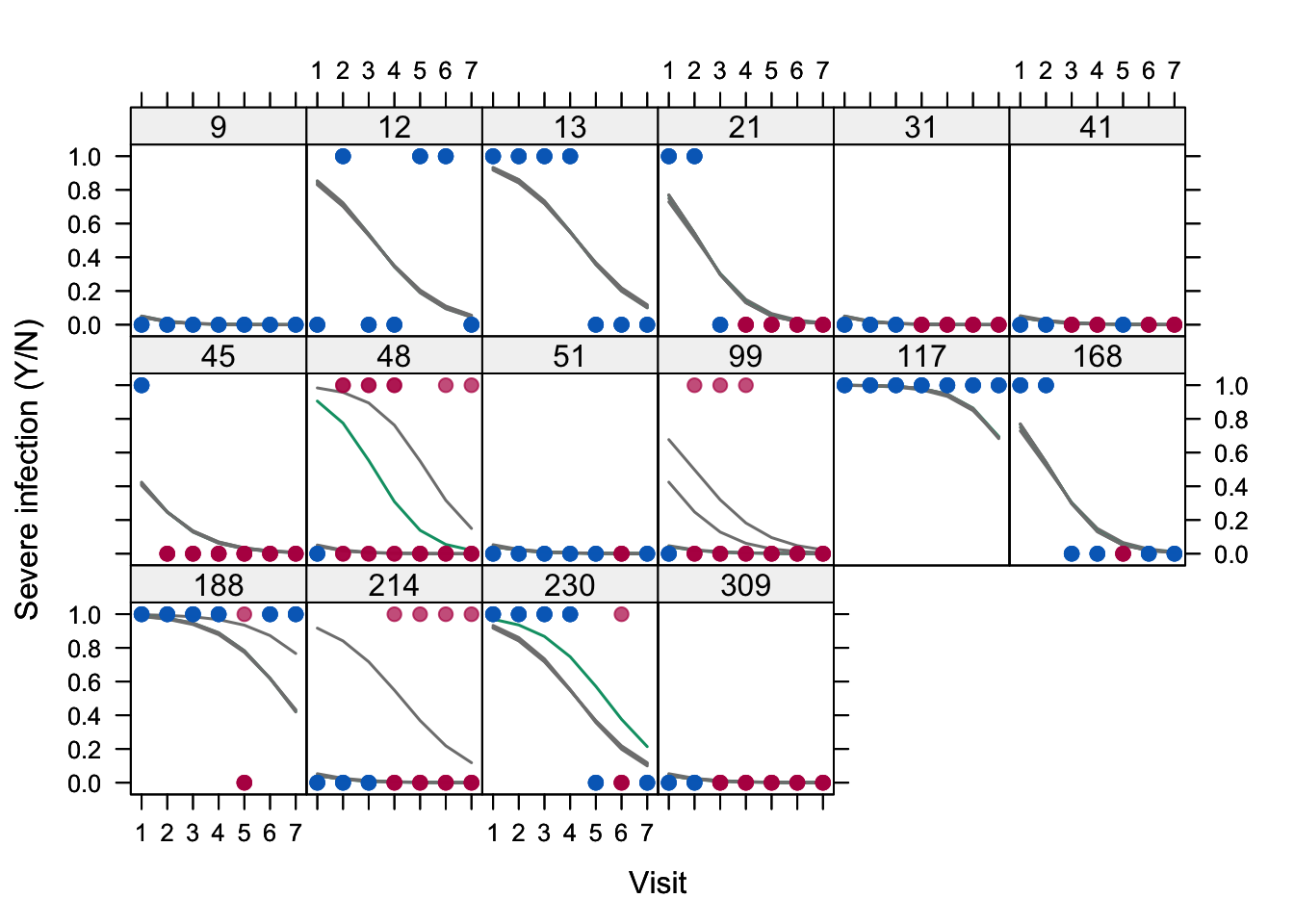 

Figure 7.4: Plot of observed (blue) and imputed (red) infection (Yes/No) by visit for 16 selected persons in the toenail data (\(m = 5\)). The lines visualize the subject-wise infection probability predicted by the generalized linear mixed model given visit, treatment and their interaction per imputed dataset.

Figure 7.4 visualizes the imputations. The plot shows the partially imputed profiles of 16 subjects in the toenail data. The general downward trend in the probability of infection severity with time is obvious, and was also found by Molenberghs and Verbeke (2005, 302). Subjects 9 (never severe) and 117 (always severe) have both complete data. They represent the extremes, and their random effect estimates are very similar in all five imputed datasets. They are close, but not identical – as you might have expected – because the multiple imputations will affect the random effects also for the fully observed subjects. Subjects 31, 41 and 309 are imputed such that their outcomes are equivalent to subject 9, and hence have similar random effect estimates. In contrast, subject 214 has the same observed data pattern as 31, but it is sometimes imputed as “severe”. As a consequence, we see that there are now two random effect estimates for this subject that are quite different, which reflects the uncertainty due to the missing data. Subjects 48 and 99 even have three clearly different estimates. Imputation number 3 is colored green instead of grey, so the isolated lines in subjects 48 and 230 come from the same imputed dataset.

The complete-data model is a generalized linear mixed model for outcome given treatment status, time and a random intercept. This is similar to the models used by Molenberghs and Verbeke (2005), but here we use the visit instead of time (which is incomplete) as the timing variable. The estimates from the combined multiple imputation analysis are then obtained as

library(purrr)
mice::complete(imp, "all") %>%
  purrr::map(lme4::glmer,
             formula = outcome ~ treatment * visit + (1 | ID),
             family = binomial) %>%
  pool() %>%
  summary()

                estimate std.error statistic  df p.value
(Intercept)       -0.937    0.5778    -1.622 546  0.1052
treatment          0.152    0.6858     0.221 941  0.8250
visit             -0.770    0.0848    -9.079 154  0.0000
treatment:visit   -0.222    0.1219    -1.826 284  0.0682

As expected, these estimates are similar to the estimates obtained from the direct analysis of these data. The added value of multiple imputation here is that it produces a dataset with scores on all visits, which makes it easier to summarize. The added values of imputation increases if important covariates are available that are not present in the substantive model, or if missing values occur in the predictors. Section 7.10.2 contains an example of that problem.