6.4 Derived variables

6.4.1 Ratio of two variables

In practice, there is often extra knowledge about the data that is not modeled explicitly. For example, consider the weight/height ratio whr, defined as wgt/hgt (kg/m). If any one of the triplet (hgt, wgt, whr) is missing, then the missing value can be calculated with certainty by a simple deterministic rule. Unless we specify otherwise, the imputation model is unaware of the relation between the three variables, and will produce imputations that are inconsistent with the rule. Inconsistent imputations are clearly undesirable since they yield combinations of data values that are impossible in the real world. Including knowledge about derived data in the imputation model prevents imputations from being inconsistent. Knowledge about the derived data can take many forms, and includes data transformations, interactions, sum scores, recoded versions, range restrictions, if-then relations and polynomials.

The easiest way to deal with the problem is to leave any derived data outside the imputation process. For example, we may impute any missing height and weight data, and append whr to the imputed data afterward. It is simple to do that in mice by

data <- boys[, c("age", "hgt", "wgt", "hc", "reg")]
imp <- mice(data, print = FALSE, seed = 71712)
long <- mice::complete(imp, "long", include = TRUE)
long$whr <- with(long, 100 * wgt / hgt)
imp.itt <- as.mids(long)

The approach is known as Impute, then transform (Von Hippel 2009). While whr will be consistent, the obvious problem with this approach is that whr is not used by the imputation method, and hence biases the estimates of parameters related to whr towards zero. Note the use of the as.mids function, which transforms the imputed data long back into a mids object.

Another possibility is to create whr before imputation, and impute whr as just another variable, known as JAV (White, Royston, and Wood 2011), or under the name Transform, then impute (Von Hippel 2009). This is easy to do, as follows:

data$whr <- 100 * data$wgt / data$hgt
imp.jav1 <- mice(data, seed = 32093, print = FALSE)

Warning: Number of logged events: 45

The warning results from the linear dependencies among the predictors, which were introduced by adding whr. The mice() function checks for linear dependencies during the iterations, and temporarily removes predictors from the univariate imputation models where needed. Each removal action is documented in the the loggedEvents component of the imp.jav1 object. The last three removal events are

tail(imp.jav1$loggedEvents, 3)

   it im dep meth out
43  5  4 whr  pmm wgt
44  5  5 wgt  pmm whr
45  5  5 whr  pmm wgt

which informs us that wgt was removed while imputing whr, and vice versa. We may prevent automatic removal by setting the relevant entries in the predictorMatrix to zero.

pred <- make.predictorMatrix(data)
pred[c("wgt", "whr"), c("wgt", "whr")] <- 0
pred[c("hgt", "whr"), c("hgt", "whr")] <- 0
pred

    age hgt wgt hc reg whr
age   0   1   1  1   1   1
hgt   1   0   1  1   1   0
wgt   1   1   0  1   1   0
hc    1   1   1  0   1   1
reg   1   1   1  1   0   1
whr   1   0   0  1   1   0

imp.jav2 <- mice(data, pred = pred, seed = 32093, print = FALSE)

This is a little faster (5-10%) and cleans out the warning.

A third approach is Passive imputation, where the transformation is done on-the-fly within the imputation algorithm. Since the transformed variable is available for imputation, the hope is that passive imputation removes the bias of the Impute, then transform methods, while restoring consistency among the imputations that was broken in JAV. Figure 6.2 visualizes the consistency of the three methods.

In mice passive imputation is invoked by specifying the tilde symbol as the first character of the imputation method. This provides a simple method for specifying dependencies among the variables, such as transformed variables, recodes, interactions, sum scores and so on. In the above example, we invoke passive imputation by

data <- boys[, c("age", "hgt", "wgt", "hc", "reg")]
data$whr <- 100 * data$wgt / data$hgt
meth <- make.method(data)
meth["whr"] <- "~I(100 * wgt / hgt)"
pred <- make.predictorMatrix(data)
pred[c("wgt", "hgt"), "whr"] <- 0
imp.pas <- mice(data, meth = meth, pred = pred,
                print = FALSE, seed = 32093)

The I() operator in the meth definitions instructs R to interpret the argument as literal. So I(100 * wgt / hgt) calculates whr by dividing wgt by hgt (in meters). The imputed values for whr are thus derived from hgt and wgt according to the stated transformation, and hence are consistent. Since whr is that last column in the data, it is updated after wgt and hgt are imputed. The changes to the default predictor matrix are needed to break any feedback loops between the derived variables and their originals. It is important to do this since otherwise whr may contain absurd imputations and the algorithm may have difficulties in convergence.

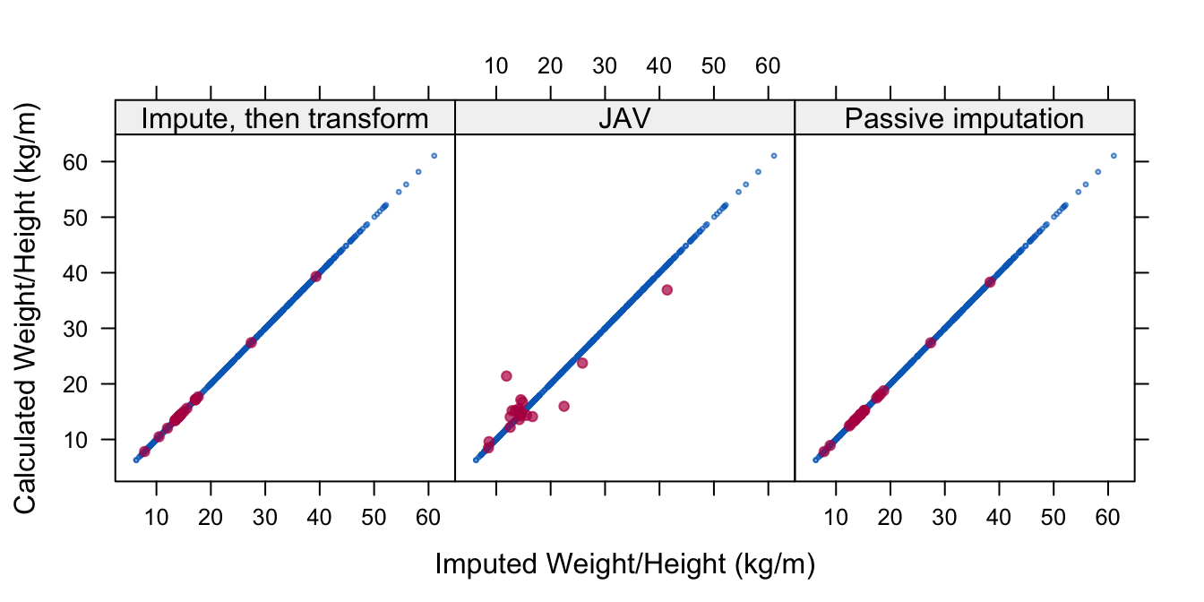
Figure 6.2: Three imputation models to impute weight/height ratio (whr). Methods Impute, then transform and Passive imputation respect the relation between whr and height (hgt) in the imputed data, whereas JAV does not.

How well do these methods impute a ratio? The simulation studies by Von Hippel (2009) and Seaman, Bartlett, and White (2012) favored the use of JAV, but neither addressed imputation of the ratio of two variables. Let us look at a small simulation comparing the three methods. As the population data, take the 681 complete records of variables age, hgt, wgt, hc and reg, and create a model for predicting height circumference from hc from more easily measured variables, including whr.

pop <- na.omit(boys[, c("age", "hgt", "wgt", "hc", "reg")])
pop$whr <- with(pop, 100 * wgt / hgt)
broom::tidy(lm(hc ~ age + hgt + wgt + whr, data = pop))

# A tibble: 5 x 5
  term        estimate std.error statistic   p.value
  <chr>          <dbl>     <dbl>     <dbl>     <dbl>
1 (Intercept)   23.7     0.656       36.1  4.25e-160
2 age           -0.308   0.0538      -5.72 1.56e-  8
3 hgt            0.176   0.00736     24.0  2.41e- 92
4 wgt           -0.496   0.0284     -17.4  1.62e- 56
5 whr            1.06    0.0583      18.2  1.22e- 60

This is a simple linear model, but the proportion of explained variance is very high, about 0.9. The ratio variable whr explains about 5% of the variance on top of the other variables. Let us randomly delete 25% of hgt and 25% of wgt, apply each of the three methods 200 times using \(m = 5\), and evaluate the parameter for whr.

Table 6.2: Evaluation of parameter for whr with 25% MCAR missing in hgt and 25% MCAR missing in wgt using four imputation strategies (\(n_\mathrm{sim} = 200\)).

Method	Bias	% Bias	Coverage	CI Width	RMSE
Impute, transform	-0.28	26.4	0.09	0.322	0.289
JAV	-0.90	84.5	0.00	0.182	0.897
Passive imputation	-0.28	26.8	0.06	0.328	0.293
smcfcs	-0.03	2.6	0.90	0.334	0.094
Listwise deletion	0.01	0.7	0.90	0.307	0.094

Table 6.2 shows that all three methods have substantial negative biases. Method JAV almost nullifies the parameter. The other two methods are better, but still far from optimal. Actually, none of these methods can be recommended for imputing a ratio.

Bartlett et al. (2015) proposed a novel rejection sampling method that creates imputations that are congenial in the sense of Meng (1994) with the substantive (complete-data) model. The method was applied to squared terms and interactions, and here we investigate whether it extends to ratios. The method has been implemented in the smcfcs package. The imputation method requires a specification of the complete-data model, as arguments smtype and smformula. An example of how to generate imputations, fit models, and pool the results is:

library(smcfcs)
data <- pop
data[sample(nrow(data), size = 100), "wgt"] <- NA
data[sample(nrow(data), size = 100), "hgt"] <- NA
data$whr <- 100 * data$wgt / data$hgt
meth <- c("", "norm", "norm", "", "", "norm")
imps <- smcfcs(originaldata = data, meth = meth, smtype = "lm",
               smformula = "hc ~ age + hgt + wgt + whr")
fit <- lapply(imps$impDatasets, lm,
              formula = hc ~ age + hgt + wgt + whr)
summary(pool(fit))

The results of the simulations are also in Table 6.2 under the heading of the smcfcs. The smcfcs method is far better than the three previous alternatives, and almost as good as one could wish for. Rejection sampling for imputation is still new and relatively unexplored, so this seems a promising area for further work.

6.4.2 Interaction terms

The standard MICE algorithm only models main effects. Sometimes the interaction between variables is of scientific interest. For example, in a longitudinal study we could be interested in assessing whether the rate of change differs between two treatment groups, in other words, the treatment-by-group interaction. The standard algorithm does not take interactions into account, so the interactions of interest should be added to the imputation model.

The usual type of interactions between two continuous variables is to subtract the mean and take the product. The following code adds an interaction betwen wgt and hc to the boys data and imputes the data by passive imputation:

expr <- expression((wgt - 40) * (hc - 50))
boys$wgt.hc <- with(boys, eval(expr))
meth <- make.method(boys)
meth["wgt.hc"] <- paste("~I(", expr, ")", sep = "")
meth["bmi"] <- ""
pred <- make.predictorMatrix(boys)
pred[c("wgt", "hc"), "wgt.hc"] <- 0
imp.int <- mice(boys, m = 1, meth = meth, pred = pred,
                print = FALSE, seed = 62587, maxit = 10)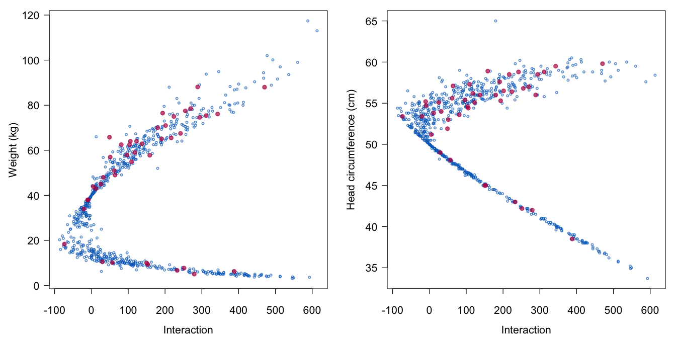

Figure 6.3: The relation between the interaction term wgt.hc (on the horizontal axes) and its components wgt and hc (on the vertical axes).

Figure 6.3 illustrates that the scatterplots of the real and synthetic values are similar. Furthermore, the imputations adhere to the stated recipe (wgt - 40) * (hc - 50). Interactions involving categorical variables can be done in similar ways (Van Buuren and Groothuis-Oudshoorn 2011), for example by imputing the data in separate groups. One may do this in mice by splitting the dataset into two or more parts, run mice() on each part and then combine the imputed datasets with rbind().

Table 6.3: Evaluation of parameter for wgt.hc with 25% MCAR missing in hc and 25% MCAR missing in wgt using four imputation strategies (\(n_\mathrm{sim} = 200\)).

Method	Bias	% Bias	Coverage	CI Width	RMSE
Impute, transform	0.20	22.7	0.17	0.290	0.207
JAV	0.63	71.5	0.00	0.229	0.632
Passive imputation	0.20	22.6	0.17	0.283	0.207
scmfcs	-0.01	0.8	0.92	0.306	0.083
Listwise deletion	-0.01	0.8	0.91	0.237	0.076

Other methods for imputing interactions are JAV, Impute, then transform and smcfcs. Table 6.3 contains the results of simulations similar to those in Section 6.4.1, but adapted to include the interaction effect shown in Figure 6.3 by using the complete-data model lm(hgt wgt + hc + wgt.hc). The results tell the same story as before, with smcfcs the best method, followed by Passive imputation and Impute, then transform.

Von Hippel (2009) stated that JAV would give consistent results under MAR, but Seaman, Bartlett, and White (2012) showed that consistency actually required MCAR. It is interesting that Seaman, Bartlett, and White (2012) found that JAV generally performed better than passive imputation, which is not confirmed in our simulations. It is not quite clear where the difference comes from, but the discussion JAV versus passive pales somewhat in the light of smcfcs.

Generic methods to preserve interactions include tree-based regression and classification (Section 3.5) as well as various joint modeling methods (Section 4.4). The relative strengths and limitations of these approaches still need to be sorted out.

6.4.3 Quadratic relations\(^\spadesuit\)

One way to analyze nonlinear relations by a linear model is to include quadratic or cubic versions of the explanatory variables into the model. Creating imputed values under such models poses some challenges. Current imputation methodology either preserves the quadratic relation in the data and biases the estimates of interest, or provides unbiased estimates but does not preserve the quadratic relation (Von Hippel 2009). It seems that we either have a congenial but misspecified model, or an uncongenial model that is specified correctly. This section describes an approach that aims to resolve this problem.

The model of scientific interest is

\[ X=\alpha + Y\beta_1 + Y^2\beta_2 + \epsilon \tag{6.1} \]

with \(\epsilon\sim N(0,\sigma^2)\). We assume that \(X\) is complete, and that \(Y=(Y_{\rm obs},Y_{\rm mis})\) is partially missing. The problem is to find imputations for \(Y\) such that estimates of \(\alpha\), \(\beta_1\), \(\beta_2\) and \(\sigma^2\) based on the imputed data are unbiased, while ensuring that the quadratic relation between \(Y\) and \(Y^2\) will hold in the imputed data.

Define the polynomial combination \(Z\) as \(Z = Y\beta_1 + Y^2\beta_2\) for some \(\beta_1\) and \(\beta_2\). The idea is to impute \(Z\) instead of \(Y\) and \(Y^2\), followed by a decomposition of the imputed data \(Z\) into components \(Y\) and \(Y^2\). Imputing \(Z\) reduces the multivariate imputation problem to a univariate problem, which is easier to manage. Under the assumption that \(P(X,Z)\) is multivariate normal, we can impute the missing part of \(Z\) by Algorithm 3.1. In cases where a normal residual distribution is suspect, we replace the linear model by predictive mean matching. The next step is to decompose \(Z\) into \(Y\) and \(Y^2\). Under the model in Equation (6.1) the value \(Y\) has two roots:

\[\begin{align} Y_- &=- { 1 \over 2\beta_2 } \left( \sqrt{4 \beta_2 Z + \beta_1^2} + \beta_1 \right)\tag{6.2}\\ Y_+ &= { 1 \over 2\beta_2 } \left( \sqrt{4\beta_2 Z + \beta_1^2} - \beta_1 \right)\tag{6.3} \end{align}\]

where we assume that the discriminant \(4\beta_2 Z + \beta_1^2\) is larger than zero. For a given \(Z\), we can take either \(Y=Y_-\) or \(Y=Y_+\), and square it to obtain \(Y^2\). Either root is consistent with \(Z = Y\beta_1 + Y^2\beta_2\), but the choice among these two options requires care. Suppose we choose \(Y_-\) for all \(Z\). Then all \(Y\) will correspond to points located on the left arm of the parabolic function. The minimum of the parabola is located at \(Y_{\rm min}=-\beta_1/2\beta_2\), so all imputations will occur in the left-hand side of the parabola. This is probably not intended.

The choice between the roots is made by random sampling. Let \(V\) be a binary random variable defined as 1 if \(Y > Y_{\rm min}\), and as 0 if \(Y \leq Y_{\rm min}\). Let us model the probability \(P(V=1)\) by logistic regression as

\[ {\rm logit} (P(V=1)) = X\psi_X + Z\psi_Z + XZ\psi_{YZ} \]

where the \(\psi\)s are parameters in the logistic regression model. Under the assumption of ignorability, we calculate the predicted probability \(P(V=1)\) from \(X_{\rm mis}\) and \(Z_{\rm mis}\). As a final step, a random draw from the binomial distribution is made, and the corresponding (negative or positive) root is selected as the imputation. This is repeated for each missing value.

---

Algorithm 6.1 (Multiple imputation of quadratic terms.\(^\spadesuit\))

1. Calculate \(Y_\mathrm{obs}^2\) for the observed \(Y\).

2. Multiply impute \(Y_\mathrm{mis}\) and \(Y_\mathrm{mis}^2\) as if they were unrelated by linear regression or predictive mean matching, resulting in imputations \(\dot Y\) and \(\dot Y^2\).

3. Estimate \(\hat\beta_1\) and \(\hat\beta_2\) by pooled linear regression of \(X\) given \(Y = (Y_\mathrm{obs},\dot Y)\) and \(Y^2 = (Y_\mathrm{obs}^2,\dot Y^2)\).

4. Calculate the polynomial combination \(Z = Y\hat\beta_1 + Y^2\hat\beta_2\).

5. Multiply impute \(Z_\mathrm{mis}\) by linear regression or predictive mean matching, resulting in imputed \(\dot Z\).

6. Calculate roots \(\dot Y_-\) and \(\dot Y_+\) given \(\hat\beta_1\), \(\hat\beta_2\) and \(\dot Z\) using Equations~ and .

7. Calculate the value on the horizontal axis at the parabolic minimum/maximum \(Y_\mathrm{min}=-\hat\beta_1/2\hat\beta_2\).

8. Calculate \(V_\mathrm{obs}=0\) if \(Y_\mathrm{obs}\leq Y_\mathrm{min}\), else \(V_{\rm obs}=1\).

9. Impute \(V_\mathrm{mis}\) by logistic regression of \(V\) given \(X\), \(Z\) and \(XZ\), resulting in imputed \(\dot V\).

10. If \(\dot V<0\) then assign \(\dot Y=\dot Y_-\), else set \(\dot Y=\dot Y_+\).

11. Calculate \(\dot Y^2\).

---

Algorithm 6.1 provides a detailed overview of all steps involved. The imputations \(\dot Z\) satisfy \(\dot Z=\dot Y\hat\beta_1+\dot Y^2\hat\beta_2\), as required. The technique is available in mice as the method quadratic. The evaluation by Vink and Van Buuren (2013) showed that the method provided unbiased estimates under four types of extreme MAR mechanisms. The idea can be generalized to polynomial bases of higher orders.

6.4.4 Compositional data\(^\spadesuit\)

Sometimes we know that a set of variables should add up to a given total. If one of the additive terms is missing, we can directly calculate its value with certainty by deducting the known terms from the total. This is known as deductive imputation (De Waal, Pannekoek, and Scholtus 2011). If two additive terms are missing, imputing one of these terms uses the available one degree of freedom, and hence implicitly determines the other term. Data of this type are known as compositional data, and they occur often in household and business surveys. Imputation of compositional data has only recently received attention (Tempelman 2007; Hron, Templ, and Filzmoser 2010; De Waal, Pannekoek, and Scholtus 2011; Vink, Lazendic, and Van Buuren 2015). Hron, Templ, and Filzmoser (2010) proposed matching on the Aitchison distance, a measure specifically designed for compositional data. The method is available in R as the robCompositions package (Templ, Hron, and Filzmoser 2011).

This section suggests a somewhat different method for imputing compositional data. Let \(Y_{123}= Y_1+Y_2+Y_3\) be the known total score of the three variables \(Y_1\), \(Y_2\) and \(Y_3\). We assume that \(Y_3\) is complete and that \(Y_1\) and \(Y_2\) are jointly missing or observed. The problem is to create multiple imputations in \(Y_1\) and \(Y_2\) such that the sum of \(Y_1\), \(Y_2\) and \(Y_3\) equals a given total \(Y_{123}\), and such that parameters estimated from the imputed data are unbiased and have appropriate coverage.

Since \(Y_3\) is known, we write \(Y_{12} = Y_{123} - Y_3\) for the sum score \(Y_1+Y_2\). The key to the solution is to find appropriate values for the ratio \(P_1 = Y_1/Y_{12}\), or equivalently for \((1-P_1)=Y_2/Y_{12}\). Let \(P(P_1|Y_1^\mathrm{obs}, Y_2^\mathrm{obs}, Y_3, X)\) denote the posterior distribution of \(P_1\), which is possibly dependent on the observed information. For each incomplete record, we make a random draw \(\dot P_1\) from this distribution, and calculate imputations for \(Y_1\) as \(\dot Y_1 = \dot P_1Y_{12}\). Likewise, imputations for \(Y_2\) are calculated by \(\dot Y_2 = (1-\dot P_1)Y_{12}\). It is easy to show that \(\dot Y_1 + \dot Y_2 = Y_{12}\), and hence \(\dot Y_1 + \dot Y_2 + Y_3 = Y_{123}\), as required.

The best way in which the posterior should be specified has still to be determined. In this section we apply standard predictive mean matching. We study the properties of the method by a small simulation study. The first step is to create an artificial dataset with known properties as follows:

set.seed(43112)
n <- 400
Y1 <- sample(1:10, size = n, replace = TRUE)
Y2 <- sample(1:20, size = n, replace = TRUE)
Y3 <- 10 + 2 * Y1 + 0.6 * Y2 + sample(-10:10, size = n,
                                      replace = TRUE)
Y <- data.frame(Y1, Y2, Y3)
Y[1:100, 1:2] <- NA
md.pattern(Y, plot = FALSE)

    Y3  Y1  Y2    
300  1   1   1   0
100  1   0   0   2
     0 100 100 200

Thus, Y is a \(400 \times 3\) dataset with 300 complete records and with 100 records in which both \(Y_1\) and \(Y_2\) are missing. Next, define three auxiliary variables that are needed for imputation:

Y123 <- Y1 + Y2 + Y3
Y12 <- Y123 - Y[,3]
P1 <- Y[,1] / Y12
data <- data.frame(Y, Y123, Y12, P1)

where the naming of the variables corresponds to the total score \(Y_{123}\), the sum score \(Y_{12}\) and the ratio \(P_1\).

The imputation model specifies how \(Y_1\) and \(Y_2\) depend on \(P_1\) and \(Y_{12}\) by means of passive imputation. The predictor matrix specifies that only \(Y_3\) and \(Y_{12}\) may be predictors of \(P_1\) in order to avoid linear dependencies.

meth <- make.method(data)
meth["Y1"]  <- "~ I(P1 * Y12)"
meth["Y2"]  <- "~ I((1 - P1) * Y12)"
meth["Y12"] <- "~ I(Y123 - Y3)"
pred <- make.predictorMatrix(data)
pred["P1", ] <- 0
pred[c("P1"), c("Y12", "Y3")] <- 1
imp1 <- mice(data, meth = meth, pred = pred, m = 10,
             print = FALSE)

The code I(P1 * Y12) calculates \(Y_1\) as the product of \(P_1\) and \(Y_{12}\), and so on. The pooled estimates are calculated as

round(summary(pool(with(imp1, lm(Y3 ~ Y1 + Y2))))[, 1:2], 2)

            estimate std.error
(Intercept)     9.71      0.98
Y1              1.99      0.11
Y2              0.61      0.05

The estimates are reasonably close to their true values of 10, 2 and 0.6, respectively. A small simulation study with these data using 100 simulations and \(m = 10\) revealed average estimates of 9.94 (coverage 0.96), 1.95 (coverage 0.95) and 0.63 (coverage 0.91). Though not perfect, the estimates are close to the truth, while the data adhere to the summation rule.

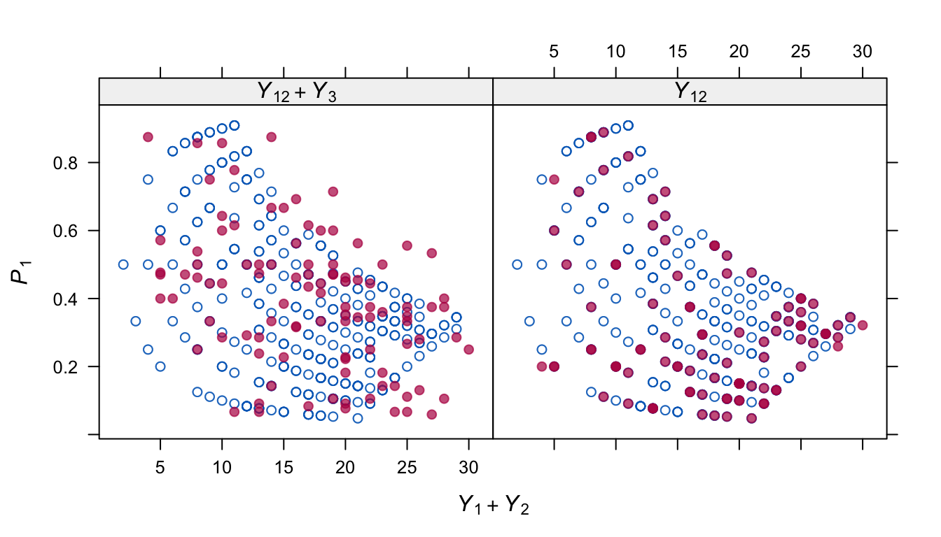
Figure 6.4: Distribution of \(P_1\) (relative contribution of \(Y_1\) to \(Y_1+Y_2\)) in the observed and imputed data at different levels of \(Y_1+Y_2\). The strong geometrical shape in the observed data is partially reproduced in the model that includes \(Y_3\).

Figure 6.4 shows where the solution might be further improved. The distribution of \(P_1\) in the observed data is strongly patterned. This pattern is only partially reflected in the imputed \(\dot P_1\) after predictive mean matching on both \(Y_{12}\) and \(Y_3\). It is possible to imitate the pattern perfectly by removing \(Y_3\) as a predictor for \(P_1\). However, this introduces bias in the parameter estimates. Evidently, some sort of compromise between these two options might further remove the remaining bias. This is an area for further research.

For a general missing data pattern, the procedure can be repeated for all pairs \((Y_j, Y_{j'})\) that have missing data. First create a consistent starting imputation that adheres to the rule of composition, then apply the above method to pairs \((Y_j, Y_{j'})\) that belong to the composition. This algorithm is a variation on the MICE algorithm with iterations occurring over pairs of variables rather than separate variables.

Vink (2015) extended these ideas to nested compositional data, where a given element of the composition is broken down into subelements. The method, called predictive ratio matching, calculates the ratio of two components, and then borrows imputations from donors that have a similar ratio. Component pairs are visited in an ingenious way and combined into an iterative algorithm.

6.4.5 Sum scores

The sum score is undefined if one of the variables to be added is missing. We can use sum scores of imputed variables within the MICE algorithm to economize on the number of predictors. For example, suppose we create a summary maturation score of the pubertal measurements gen, phb and tv, and use that score to impute the other variables instead of the three original pubertal measurements.

Another area of application is the imputation of test items that form a scale. When the number of items is small relative to the sample size, good results can be obtained by imputing the items in a full imputation model, where all items are used to impute others (Van Buuren 2010). This method becomes unfeasible for a larger number of items. In that case, one may structure the imputation problem assuming one knows which items belong to which scale. Suppose that the data consist of an outcome variable out, a background variable bck, a scale a with ten items a1-a10, a scale b with twelve items b1-b12, and that all variables contain missing values. After filling in starting imputations, the imputation model would take the following steps:

1. Impute out given bck, a, b, where a and b are the summed scale scores from b1-b10 and b1-b12;

2. Impute bck given out, a and b;

3. Impute a1 given out, bck, b and a2-a10;

4. Impute a2 given out, bck, b and a1, a3-a10;

5. Impute a3-a10 along the same way;

6. Impute b1 given out, bck, a and b2-b12, where a is the updated summed scale score;

7. Impute b2-b12 along the same way.

This technique will condense the imputation model, so that it will become both faster and more stable. It is easy to specify such models in mice. See Van Buuren and Groothuis-Oudshoorn (2011) for examples.

Plumpton et al. (2016) found that the technique reduced the standard error on average by 39% compared to complete-case analysis, resulting in more precise conclusions. Eekhout et al. (2018) found that the technique outperforms existing techniques (complete-case analysis, imputing only total scores) with respect to bias and efficiency. As an alternative, one may use the mean of the observed items as the scale score (the parcel summary), which is easier than calculating the total score. Both studies obtained results that were comparable to using the total score. Note that the parcel summary mean requires the assumption that the missing items are MCAR, which may be problematic for speeded tests and for scales where items increase in difficulty. The magnitude of the effect of violations of the MCAR assumption on bias is still to be determined.

6.4.6 Conditional imputation

In some cases it makes sense to restrict the imputations, possibly conditional on other data. The method in Section 1.3.5 produced negative values for the positive-valued variable Ozone. One way of dealing with this mismatch between the imputed and observed values is to censor the values at some specified minimum or maximum value. The mice() function has an argument called post that takes a vector of strings of R commands. These commands are parsed and evaluated just after the univariate imputation function returns, and thus provide a way to post-process the imputed values. Note that post only affects the synthetic values, and leaves the observed data untouched. The squeeze() function in mice replaces values beyond the specified bounds by the minimum and maximal scale values. A hacky way to ensure positive imputations for Ozone under stochastic regression imputation is

data <- airquality[, 1:2]
post <- make.post(data)
post["Ozone"] <-
  "imp[[j]][, i] <- squeeze(imp[[j]][, i], c(1, 200))"
imp <- mice(data, method = "norm.nob", m = 1,
            maxit = 1, seed = 1, post = post)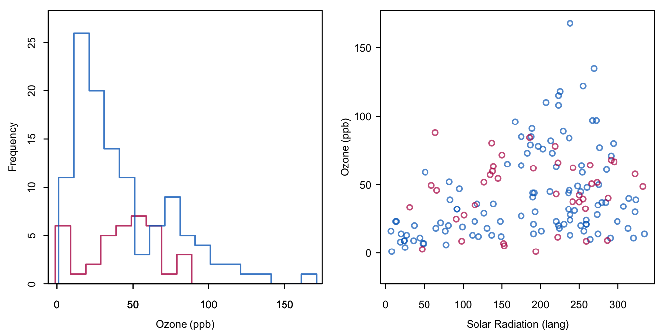

Figure 6.5: Stochastic regression imputation of Ozone, where the imputed values are restricted to the range 1–200. Compare to Figure 1.4.

Compare Figure 6.5 to Figure 1.4. The negative ozone value of -18.8 has now been replaced by a value of 1.

The previous syntax of the post argument is a bit cumbersome. The same result can be achieved by neater code:

post["Ozone"] <- "ifdo(c(Ozone < 1, Ozone > 200), c(1, 200))"

The ifdo() function is a convenient way to create conditional imputes. For example, in the boys data puberty is measured only for boys older than 8 years. Before this age it is unlikely that puberty has started. It is a good idea to bring this extra information into the imputation model to stabilize the solution. More precisely, we may restrict any imputations of gen, phb and tv to the lowest possible category for those boys younger than 8 years. This can be achieved by

post <- make.post(boys)
post["gen"] <-
  "imp[[j]][data$age[!r[, j]] < 8, i] <- levels(boys$gen)[1]"
post["phb"] <-
  "imp[[j]][data$age[!r[, j]] < 8, i] <- levels(boys$phb)[1]"
post["tv"]  <- "imp[[j]][data$age[!r[, j]] < 8, i] <- 1"
free <- mice(boys, m = 1, seed = 85444, print = FALSE)
restricted <- mice(boys, m = 1, post = post, seed = 85444,
                   print = FALSE)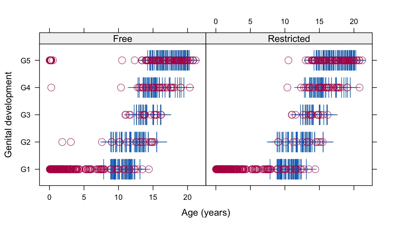

Figure 6.6: Genital development of Dutch boys by age. The free solution does not constrain the imputations, whereas the restricted solution requires all imputations below the age of 8 years to be at the lowest category.

Figure 6.6 compares the scatterplot of genital development against age for the free and restricted solutions. Around infancy and early childhood, the imputations generated under the free solution are clearly unrealistic due to the severe extrapolation of the data between the ages 0–8 years. The restricted solution remedies this situation by requiring that pubertal development does not start before the age of 8 years.

The post-processing facility provides almost limitless possibilities to customize the imputed values. For example, we could reset the imputed value in some subset of the missing data to NA, thus imputing only some of the variables. Of course, appropriate care is needed when using this partially imputed variable later on as a predictor. Another possibility is to add or multiply the imputed data by a given constant in the context of a sensitivity analysis for nonignorable missing data mechanisms (see Section 3.8). More generally, we might re-impute some entries in the dataset depending on their current value, thus opening up possibilities to specify methods for nonignorable missing data.