10.2 Correcting for nonresponse

This section describes how multiple imputation can be used to “make a sample representative.” Weighting to known population totals is widely used to correct for nonresponse (Bethlehem 2002; Särndal and Lundström 2005). Imputation is an alternative to weighting. Imputation provides fine-grained control over the correction process. Provided that the imputation method is confidence proper, estimation of the correct standard errors can be done using Rubin’s rules. Note however that this is not without controversy: Marker, Judkins, and Winglee (2002, 332) criticize multiple imputation as “difficult to apply,” “to require massive amounts of computation,” and question its performance for clustered datasets and unplanned analyses. Weighting and multiple imputation can also be combined, as was done in the NHANES III imputation project (Khare et al. 1993; Schafer et al. 1996).

This section demonstrates an application in the situation where the nonresponse is assumed to depend on known covariates, and where the distribution of covariates in the population is known. The sample is augmented by a set of artificial records, the outcomes in this set are multiply imputed and the whole set is analyzed. Though the application assumes random sampling, it should not be difficult to extend the basic ideas to more complex sampling designs.

10.2.1 Fifth Dutch Growth Study

The Fifth Dutch Growth Study is a cross-sectional nationwide study of height, weight and other anthropometric measurements among children 0-21 years living in the Netherlands (Schönbeck et al. 2013). The goal of the study is to provide updated growth charts that are representative for healthy children. The study is an update of similar studies performed in the Netherlands in 1955, 1965, 1980 and 1997. A strong secular trend in height has been observed over the last 150 years, making the Dutch population the tallest in the world (Fredriks, Van Buuren, Burgmeijer, et al. 2000). The growth studies yield essential information needed to calibrate the growth charts for monitoring childhood growth and development. One of the parameters of interest is final height, the mean height of the population when fully grown around the age of 20 years.

The survey took place between May 2008 and October 2009. The sample was stratified into five regions: North (Groningen, Friesland, Drenthe), East (Overijssel, Gelderland, Flevoland), West (Noord-Holland, Zuid-Holland, Utrecht), South (Zeeland, Noord-Brabant, Limburg) and the four major cities (Amsterdam, Rotterdam, The Hague, Utrecht City). The way in which the children were sampled depended on age. Up to 8 years of age, measurements were performed during regular periodical health examinations. Children older than 9 years were sampled from the population register, and received a personal invitation from the local health care provider.

The total population was stratified into three ethnic subpopulations. Here we consider only the subpopulation of Dutch descent. This group consists of all children whose biological parents are born in the Netherlands. Children with growth-related diseases were excluded. The planned sample size for the Dutch subpopulation was equal to 14782.

10.2.2 Nonresponse

During data collection, it quickly became evident that the response in children older than 15 years was extremely poor, and sometimes fell even below 20%. Though substantial nonresponse was caused by lack of perceived interest by the children, we could not rule out the possibility of selective nonresponse. For example, overweight children may have been less inclined to participate. The data collection method was changed in November 2008 so that all children with a school class were measured. Once a class was selected, nonresponse of the pupils was very generally small. In addition, children were measured by special teams at two high schools, two universities and a youth festival. The sample was supplemented with data from two studies from Amsterdam and Zwolle.

10.2.3 Comparison to known population totals

The realized sample size was \(n\) = 10030 children aged 0-21 years (4829 boys, 5201 girls). The nonresponse and the changes in the design may have biased the sample. If the sample is to be representative for the Netherlands, then the distribution of measured covariates like age, sex, region or educational level should conform to known population totals. Such population totals are based on administrative sources and are available in STATLINE, the online publication system of Statistics Netherlands.

Table 10.3: Distribution of the population and the sample over five geographical regions by age. Numbers are column percentages. Source: Fifth Dutch Growth Study (Schönbeck et al. 2013).

	0-9 yrs		10-13 yrs		14-21 yrs
Region	Population	Sample	Population	Sample	Population	Sample
North	12	7	12	11	12	4
East	24	28	24	11	24	55
South	23	27	24	31	25	21
West	21	26	20	26	20	15
City	20	12	19	22	19	4

Table 10.3 compares the proportion of children within five geographical regions in the Netherlands per January 1, 2010, with the proportions in the sample. Geography is known to be related to height, with the 20-year-olds in the North being about 3cm taller in the North (Fredriks, Van Buuren, Burgmeijer, et al. 2000). There are three age groups. In the youngest children, the population and sample proportions are reasonably close in the East, South and West, but there are too few children from the North and the major cities. For children aged 10-13 years, there are too few children from the North and East. In the oldest children, the sample underrepresents the North and the major cities, and overrepresents the East.

10.2.4 Augmenting the sample

Table 10.4: Number of observed and imputed children in the sample by geographical regions and age. Source: Fifth Dutch Growth Study (Schönbeck et al. 2013).

	0-9 yrs		10-13 yrs		14-21 yrs
Region	\(n_{\rm obs}\)	\(n_{\rm imp}\)	\(n_{\rm obs}\)	\(n_{\rm imp}\)	\(n_{\rm obs}\)	\(n_{\rm imp}\)
North	389	400	200	75	143	200
East	1654	0	207	300	667	0
South	1591	0	573	0	767	0
West	1530	0	476	0	572	0
City	696	600	401	0	164	400
Total	5860	1000	1857	375	2313	600

The idea is to augment the sample in such a way that it will be nationally representative, followed by multiple imputation of the outcomes of interest. Table 10.4 lists the number of the measured children. The table also reports the number of children needed to bring the sample close to the population distribution.

In total 1975 records are appended to the 10030 records of children who were measured. The appended data contain three complete covariates: region, sex and age in years. For example, for the combination (North, 0-9 years) \(n_{\rm imp}\) = 400 new records are created as follows. All 400 records have the region category North. The first 200 records are boys and the last 200 records are girls. Age is drawn uniformly from the range 0-9 years. The outcomes of interest, like height and weight, are set to missing. Similar blocks of records are created for the other five categories of interest, resulting in a total of 1975 new records with complete covariates and missing outcomes.

The following R code creates a dataset of 1975 records, with four complete covariates (id, reg, sex, age) and four missing outcomes (hgt, wgt, hgt.z, wgt.z). The outcomes hgt.z and wgt.z are standard deviation scores (SDS), or \(Z\)-scores, derived from hgt and wgt, respectively, standardized for age and sex relative to the Dutch references (Fredriks, Van Buuren, Burgmeijer, et al. 2000).

nimp <- c(400, 600, 75, 300, 200, 400)
regcat <- c("North", "City", "North", "East", "North", "City")
reg <- rep(regcat, nimp)
nimp2 <- floor(rep(nimp, each = 2)/2)
nimp2[5:6] <- c(38, 37)
sex <- rep(rep(c("boy", "girl"), 6), nimp2)
minage <- rep(c(0, 0, 10, 10, 14, 14), nimp)
maxage <- rep(c(10, 10, 14, 14, 21, 21), nimp)
set.seed(42444)
age <- runif(length(minage), minage, maxage)
id <- 600001:601975
data("fdgs", package = "mice")
pad <- data.frame(id, reg, age, sex,
                  hgt = NA, wgt = NA, hgt.z = NA, wgt.z = NA)
data <- rbind(fdgs, pad)

10.2.5 Imputation model

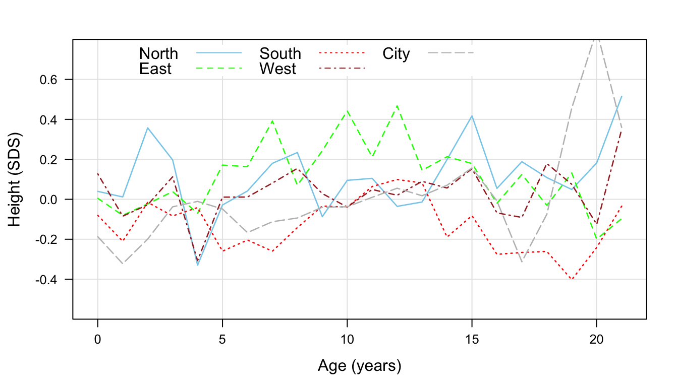
Figure 10.5: Height SDS by age and region of Dutch children. Source: Fifth Dutch Growth Study (\(n\) = 10030).

Regional differences in height are not constant across age, and tend to be more pronounced in older children. Figure 10.5 displays mean height standard deviation scores by age and region. Children from the North are generally the tallest, while those from the South are shortest, but the difference varies somewhat with age. Children from the major cities are short at early ages, but relatively tall in the oldest age groups. Imputation should preserve these features in the data, so we need to include at least the age by region interaction into the imputation model. In addition, we incorporate the interaction between SDS and age, so that the relation between height and weight could differ across age. The following specification uses the new formulas argument of mice to specify the interaction terms. This setup eliminates the need for passive imputation.

form <- list(hgt.z ~ reg + age + sex + wgt.z +
               I((age - 10) * wgt.z) + age * reg,
             wgt.z ~ reg + age + sex + hgt.z +
               I((age - 10) * hgt.z) + age * reg)
imp <- mice(data, meth = "norm", form = form, m = 10,
            maxit = 20, seed = 28107, print = FALSE)

Height SDS and weight SDS are is approximately normally distributed with a mean of zero and a standard deviation of 1, so we use the linear normal model method norm rather the pmm. If necessary, absolute values in centimeters (cm) and kilograms (kg) can be calculated after imputation.

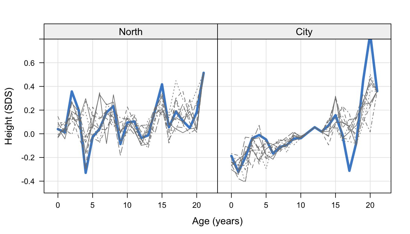
Figure 10.6: Mean height SDS by age for regions North and City, in the observed data (\(n\) = 10030) (blue) and 10 augmented datasets that correct for the nonresponse (\(n\) = 12005).

Figure 10.6 displays mean height SDS per year for regions North and City in the original and augmented data. The 10 imputed datasets show patterns in mean height SDS similar to those in the observed data. Because of the lower sample size, the means for region North are more variable than City. Observe also that the rising pattern in City is reproduced in the imputed data. No imputations were generated for the ages 10-13 years, which explains that the means of the imputed and observed data coincide. The imputations tend to smooth out sharp peaks at higher ages due to the low number of data points.

10.2.6 Influence of nonresponse on final height

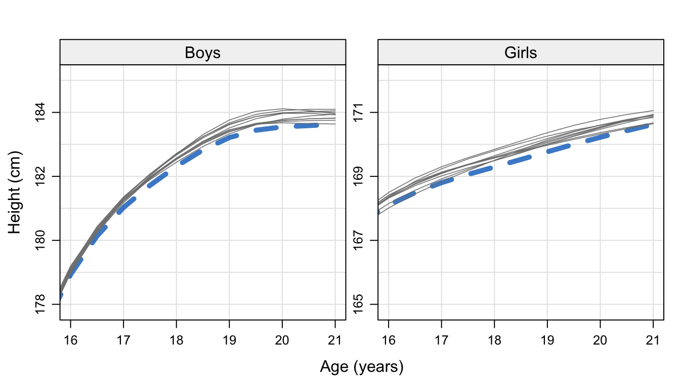
Figure 10.7: Final height estimates in Dutch boys and girls from the original sample (\(n\) = 10030) and 10 augmented samples (\(n\) = 12005) that correct for the nonresponse.

Figure 10.7 displays the mean of fitted height distribution of the original and the 10 imputed datasets. Since children from the shorter population in the South are overrepresented, the estimates of final height from the sample (183.6 cm for boys, 170.6 cm for girls) are biased downward. The estimates calculated from the imputed data vary from 183.6 to 184.1 cm (boys) and 170.6 to 171.1 cm (girls). Thus, correcting for the nonresponse leads to final height estimates that are about 2 mm higher.

10.2.7 Discussion

The application as described here only imputes height and weight in Dutch children. It is straightforward to extend the method to impute additional outcomes, like waist or hip circumference.

The method can only correct for covariates whose distributions are known in both the sample and population. It does not work if nonresponse depends on factors for which we have no population distribution. However, if we have possession of nonresponse forms for a representative sample, we may use any covariates common to the responders and nonresponders to correct for the nonresponse using a similar methodology. The correction will be more successful if these covariates are related to the reasons for the nonresponse.

There are no accepted methods yet to calculate the number of extra records needed. Here we used 1975 new records to augment the existing 10030 records, about 16% of the total. This number of artificial records brought the covariate distribution in the augmented sample close to the population distribution without the need to discard any of the existing records. When the imbalance grows, we may need a higher percentage of augmentation. The estimates will then be based on a larger fraction of missing information, and may thus become unstable. Alternatively, we could sacrifice some of the existing records by taking a random subsample of strata that are overrepresented, but discarding data is likely to lead it less efficient estimates. It would be interesting to compare the methodology to traditional weighting approaches.