1.3 Ad-hoc solutions
1.3.1 Listwise deletion
Complete-case analysis (listwise deletion) is the default way of handling incomplete data in many statistical packages, including SPSS, SAS and Stata. The function na.omit() does the same in S-PLUS and R. The procedure eliminates all cases with one or more missing values on the analysis variables. An important advantage of complete-case analysis is convenience. If the data are MCAR, listwise deletion produces unbiased estimates of means, variances and regression weights. Under MCAR, listwise deletion produces standard errors and significance levels that are correct for the reduced subset of data, but that are often larger relative to all available data.
A disadvantage of listwise deletion is that it is potentially wasteful. It is not uncommon in real life applications that more than half of the original sample is lost, especially if the number of variables is large. King et al. (2001) estimated that the percentage of incomplete records in the political sciences exceeded 50% on average, with some studies having over 90% incomplete records. It will be clear that a smaller subsample could seriously degrade the ability to detect the effects of interest.
If the data are not MCAR, listwise deletion can severely bias estimates of means, regression coefficients and correlations. Little and Rubin (2002, 41–44) showed that the bias in the estimated mean increases with the difference between means of the observed and missing cases, and with the proportion of the missing data. Schafer and Graham (2002) reported an elegant simulation study that demonstrates the bias of listwise deletion under MAR and MNAR. However, complete-case analysis is not always bad. The implications of the missing data are different depending on where they occur (outcomes or predictors), and the parameter and model form of the complete-data model. In the context of regression analysis, listwise deletion possesses some unique properties that make it attractive in particular settings. There are cases in which listwise deletion can provide better estimates than even the most sophisticated procedures. Since their discussion requires a bit more background than can be given here, we defer the treatment to Section 2.7.
Listwise deletion can introduce inconsistencies in reporting. Since listwise deletion is automatically applied to the active set of variables, different analyses on the same data are often based on different subsamples. In principle, it is possible to produce one global subsample using all active variables. In practice, this is unattractive since the global subsample will always have fewer cases than each of the local subsamples, so it is common to create different subsets for different tables. It will be evident that this complicates their comparison and generalization to the study population.
In some cases, listwise deletion can lead to nonsensical subsamples. For example, the rows in the airquality dataset used in Section 1.1.1 correspond to 154 consecutive days between May 1, 1973 and September 30, 1973. Deleting days affects the time basis. It would be much harder, if not impossible, to perform analyses that involve time, e.g., to identify weekly patterns or to fit autoregressive models that predict from previous days.
The opinions on the merits of listwise deletion vary. Miettinen (1985, 231) described listwise deletion as
…the only approach that assures that no bias is introduced under any circumstances…
a bold statement, but incorrect. At the other end of the spectrum we find Enders (2010, 39):
In most situations, the disadvantages of listwise deletion far outweigh its advantages.
Schafer and Graham (2002, 156) cover the middle ground:
If a missing data problem can be resolved by discarding only a small part of the sample, then the method can be quite effective.
The leading authors in the field are, however, wary of providing advice about the percentage of missing cases below which it is still acceptable to do listwise deletion. Little and Rubin (2002) argue that it is difficult to formulate rules of thumb since the consequences of using listwise deletion depend on more than the missing data rate alone. Vach (1994, 113) expressed his dislike for simplistic rules as follows:
It is often supposed that there exists something like a critical missing rate up to which missing values are not too dangerous. The belief in such a global missing rate is rather stupid.
1.3.2 Pairwise deletion
Pairwise deletion, also known as available-case analysis, attempts to remedy the data loss problem of listwise deletion. The method calculates the means and (co)variances on all observed data. Thus, the mean of variable \(X\) is based on all cases with observed data on \(X\), the mean of variable \(Y\) uses all cases with observed \(Y\)-values, and so on. For the correlation and covariance, all data are taken on which both \(X\) and \(Y\) have non-missing scores. Subsequently, the matrix of summary statistics are fed into a program for regression analysis, factor analysis or other modeling procedures.
SPSS, SAS and Stata contain many procedures with an option for pairwise deletion. In R we can calculate the means and correlations of the airquality data under pairwise deletion in R as:
data <- airquality[, c("Ozone", "Solar.R", "Wind")]
mu <- colMeans(data, na.rm = TRUE)
cv <- cov(data, use = "pairwise")
The standard lm() function does not take means and covariances as input, but the lavaan package (Rosseel 2012) provides this feature:
library(lavaan)
fit <- lavaan("Ozone ~ 1 + Wind + Solar.R
              Ozone ~~ Ozone",
             sample.mean = mu, sample.cov = cv,
             sample.nobs = sum(complete.cases(data)))
The method is simple, and appears to use all available information. Under MCAR, it produces consistent estimates of mean, correlations and covariances (Little and Rubin 2002, 55). The method has also some shortcomings. First, the estimates can be biased if the data are not MCAR. Further, the covariance and/or correlation matrix may not be positive definite, which is requirement for most multivariate procedures. Problems are generally more severe for highly correlated variables (Little 1992). It is not clear what sample size should be used for calculating standard errors. Taking the average sample size yields standard errors that are too small(Little 1992). Also, pairwise deletion requires numerical data that follow an approximate normal distribution, whereas in practice we often have variables of mixed types.
The idea to use all available information is good, but the proper analysis of the pairwise matrix requires sophisticated optimization techniques and special formulas to calculate the standard errors (Van Praag, Dijkstra, and Van Velzen 1985; Marsh 1998), which somewhat defeats its utility. Pairwise deletion works best used if the data approximate a multivariate normal distribution, if the correlations between the variables are low, and if the assumption of MCAR is plausible. It is not recommended for other cases.
1.3.3 Mean imputation
A quick fix for the missing data is to replace them by the mean. We may use the mode for categorical data. Suppose we want to impute the mean in Ozone and Solar.R of the airquality data. SPSS, SAS and Stata have pre-built functions that substitute the mean. This book uses the R package mice (Van Buuren and Groothuis-Oudshoorn 2011). This software is a contributed package that extends the functionality of R. Before mice can be used, it must be installed. An easy way to do this is to type:
install.packages("mice")which searches the Comprehensive R Archive Network (CRAN), and installs the requested package on the local computer. After succesful installation, the mice package can be loaded by
library("mice")Imputing the mean in each variable can now be done by
imp <- mice(airquality, method = "mean", m = 1, maxit = 1)
 iter imp variable
  1   1  Ozone  Solar.R
The argument method = mean specifies mean imputation, the argument m = 1 requests a single imputed dataset, and maxit = 1 sets the number of iterations to 1 (no iteration). The latter two options can be left to their defaults with essentially the same result.
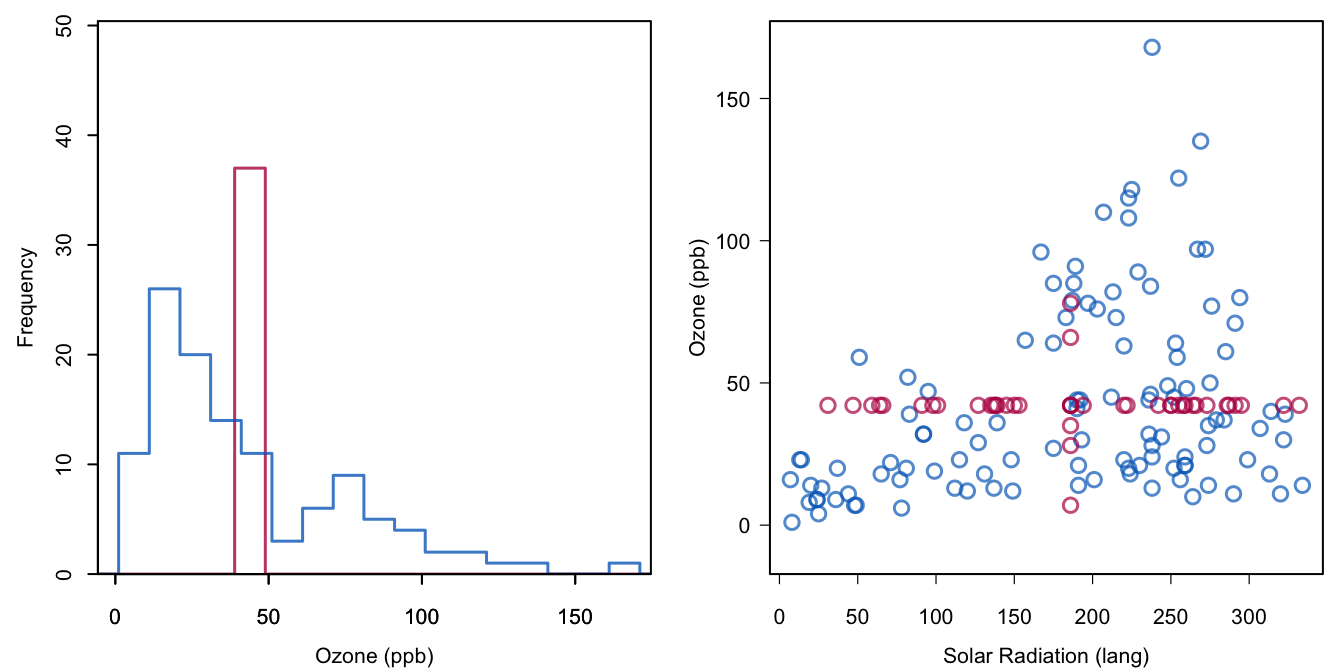
Figure 1.2: Mean imputation of Ozone. Blue indicates the observed data, red indicates the imputed values.
Mean imputation distorts the distribution in several ways. Figure 1.2 displays the distribution of Ozone after imputation. In the figure on the left, the red bar at the mean stands out. Imputing the mean here actually creates a bimodal distribution. The standard deviation in the imputed data is equal to 28.7, much smaller than from the observed data alone, which is 33. The figure on the right-hand side shows that the relation between Ozone and Solar.R is distorted because of the imputations. The correlation drops from 0.35 in the blue points to 0.3 in the combined data.
Mean imputation is a fast and simple fix for the missing data. However, it will underestimate the variance, disturb the relations between variables, bias almost any estimate other than the mean and bias the estimate of the mean when data are not MCAR. Mean imputation should perhaps only be used as a rapid fix when a handful of values are missing, and it should be avoided in general.
1.3.4 Regression imputation
Regression imputation incorporates knowledge of other variables with the idea of producing smarter imputations. The first step involves building a model from the observed data. Predictions for the incomplete cases are then calculated under the fitted model, and serve as replacements for the missing data. Suppose that we predict Ozone by linear regression from Solar.R.
fit <- lm(Ozone ~ Solar.R, data = airquality)
pred <- predict(fit, newdata = ic(airquality))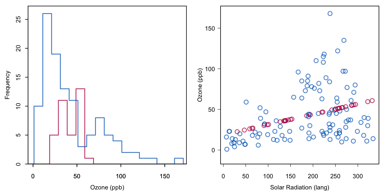
Figure 1.3: Regression imputation: Imputing Ozone from the regression line.
Another possibility for regression imputation uses mice:
data <- airquality[, c("Ozone", "Solar.R")]
imp <- mice(data, method = "norm.predict", seed = 1,
           m = 1, print = FALSE)
xyplot(imp, Ozone ~ Solar.R)
Figure 1.3 shows the result. The imputed values correspond to the most likely values under the model. However, the ensemble of imputed values vary less than the observed values. It may be that each of the individual points is the best under the model, but it is very unlikely that the real (but unobserved) values of Ozone would have had this distribution. Imputing predicted values also has an effect on the correlation. The red points have a correlation of 1 since they are located on a line. If the red and blue dots are combined, then the correlation increases from 0.35 to 0.39. Note that this upward bias grows with the percent missing ozone levels (here 24%).
Regression imputation yields unbiased estimates of the means under MCAR, just like mean imputation, and of the regression weights of the imputation model if the explanatory variables are complete. Moreover, the regression weights are unbiased under MAR if the factors that influence the missingness are part of the regression model. In the example this corresponds to the situation where Solar.R would explain any differences in the probability that Ozone is missing. On the other hand, correlations are biased upwards, and the variability of the imputed data is systematically underestimated. The degree of underestimation depends on the explained variance and on the proportion of missing cases (Little and Rubin 2002, 64).
Imputing predicted values can yield realistic imputations if the prediction is close to perfection. If so, the method reconstructs the missing parts from the available data. In essence, there was not really any information missing in the first place, it was only coded in a different form.
Regression imputation, as well as its modern incarnations in machine learning is probably the most dangerous of all methods described here. We may be led to believe that we’re to do a good job by preserving the relations between the variables. In reality however, regression imputation artificially strengthens the relations in the data. Correlations are biased upwards. Variability is underestimated. Imputations are too good to be true. Regression imputation is a recipe for false positive and spurious relations.
1.3.5 Stochastic regression imputation
Stochastic regression imputation is a refinement of regression imputation attempts to address correlation bias by adding noise to the predictions. The following code imputes Ozone from Solar.R by stochastic regression imputation.
data <- airquality[, c("Ozone", "Solar.R")]
imp <- mice(data, method = "norm.nob", m = 1, maxit = 1,
            seed = 1, print = FALSE)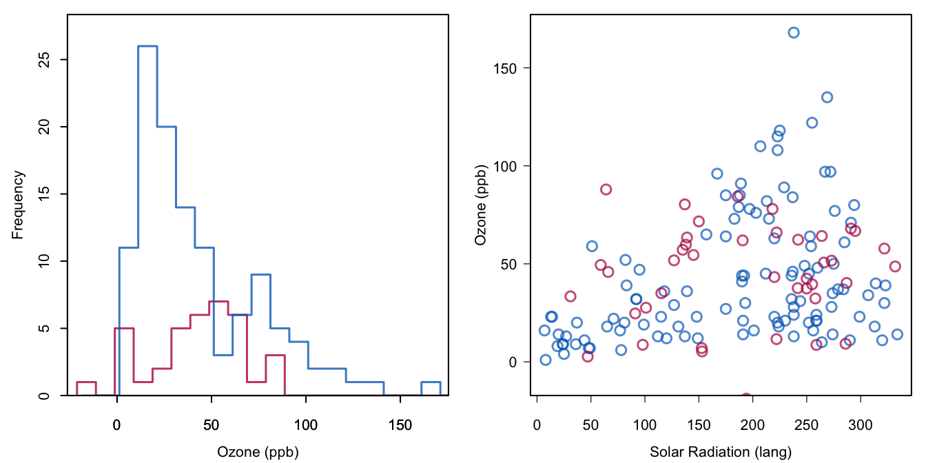
Figure 1.4: Stochastic regression imputation of Ozone.
The method = norm.nob argument requests a plain, non-Bayesian, stochastic regression method. This method first estimates the intercept, slope and residual variance under the linear model, then calculates the predicted value for each missing value, and adds a random draw from the residual to the prediction. We will come back to the details in Section 3.2. The seed argument makes the solution reproducible. Figure 1.4 shows that the addition of noise to the predictions opens up the distribution of the imputed values, as intended.
Note that some new complexities arise. There is one imputation with a negative value. Such values need not be due to the draws from the residual distribution, but can also be a consequence of the use of a linear model for non-negative data. In fact, Figure 1.1 shows several negative predicted values in the observed data. Since negative Ozone concentrations do not exist in the real world, we cannot consider negative values as plausible imputations. Note also that the high end of the distribution is not well covered. The observed data form a cone, i.e., the data are heteroscedastic, but the imputation model assumes equal dispersion around the regression line. The variability of Ozone increases up to the solar radiation level of 250 langleys, and decreases after that. Though it is unclear whether this is a genuine meteorological phenomenon, the imputation model does not account for this feature.
Nevertheless, stochastic regression imputation represents a major conceptual advance. Some analysts may find it counterintuitive to “spoil” the best prediction by adding random noise, yet this is precisely what makes it suitable for imputation. A well-executed stochastic regression imputation preserves not only the regression weights, but also the correlation between variables (cf. Exercise 1.3). The main idea to draw from the residuals is very powerful, and forms the basis of more advanced imputation techniques.
1.3.6 LOCF and BOCF
Last observation carried forward (LOCF) and baseline observation carried forward (BOCF) are ad-hoc imputation methods for longitudinal data. The idea is to take the previous observed value as a replacement for the missing data. When multiple values are missing in succession, the method searches for the last observed value.
The function fill() from the tidyr package applies LOCF by filling in the last known value. This is useful in situations where values are recorded only as they change, as in time-to-event data. For example, we may use LOCF to fill in Ozone by
airquality2 <- tidyr::fill(airquality, Ozone)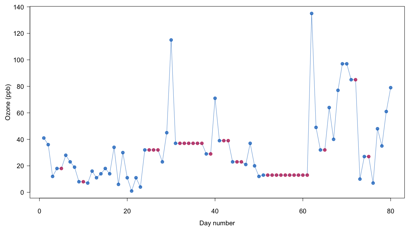
Figure 1.5: Imputation of Ozone by last observation carried forward (LOCF).
Figure 1.5 plots the results of the first 80 days of the Ozone series. The stretches of red dots indicate the imputations, and are constant within the same batch of missing ozone levels. The real, unseen values are likely to vary within these batches, so applying LOCF here gives implausible imputations.
LOCF is convenient because it generates a complete dataset. It can be applied with confidence in cases where we are certain what the missing values should be, for example, for administrative variables in longitudinal data. For outcomes, LOCF is dubious. The method has long been used in clinical trials. The U.S. Food and Drug Administration (FDA) has traditionally viewed LOCF as the preferred method of analysis, considering it conservative and less prone to selection than listwise deletion. However, Molenberghs and Kenward (2007, 47–50) show that the bias can operate in both directions, and that LOCF can yield biased estimates even under MCAR. LOCF needs to be followed by a proper statistical analysis method that distinguishes between the real and imputed data. This is typically not done however. Additional concerns about a reversal of the time direction are given in Kenward and Molenberghs (2009).
The Panel on Handling Missing Data in Clinical Trials recommends that LOCF and BOCF should not be used as the primary approach for handling missing data unless the assumptions that underlie them are scientifically justified (National Research Council 2010, 77).
1.3.7 Indicator method
Suppose that we want to fit a regression, but there are missing values in one of the explanatory variables. The indicator method (Miettinen 1985, 232) replaces each missing value by a zero and extends the regression model by the response indicator. The procedure is applied to each incomplete variable. The user analyzes the extended model instead of the original.
In R the indicator method can be coded as
imp <- mice(airquality, method = "mean", m = 1,
            maxit = 1, print = FALSE)
airquality2 <- cbind(complete(imp),
                     r.Ozone = is.na(airquality[, "Ozone"]))
fit <- lm(Wind ~ Ozone + r.Ozone, data = airquality2)
Observe that since the missing data are in Ozone we needed to reverse the direction of the regression model.
The indicator method has been popular in public health and epidemiology. An advantage is that the indicator method retains the full dataset. Also, it allows for systematic differences between the observed and the unobserved data by inclusion of the response indicator, and could be more efficient. White and Thompson (2005) pointed out that the method can be useful to estimate the treatment effect in randomized trials when a baseline covariate is partially observed. If the missing data are restricted to the covariate, if the interest is solely restricted to estimation of the treatment effect, if compliance to the allocated treatment is perfect and if the model is linear without interactions, then using the indicator method for that covariate yields an unbiased estimate of the treatment effect. This is true even if the missingness depends on the covariate itself. Additional work can be found in Groenwold et al. (2012; Sullivan et al. 2018). It is not yet clear whether the coverage of the confidence interval around the treatment estimate will be satisfactory for multiple incomplete baseline covariates.
The conditions under which the indicator method works may not be met in practice. For example, the method does not allow for missing data in the outcome, and generally fails in observational data. It has been shown that the method can yield severely biased regression estimates, even under MCAR and for low amounts of missing data (Vach and Blettner 1991; Greenland and Finkle 1995; Knol et al. 2010). The indicator method may have its uses in particular situations, but fails as a generic method to handle missing data.
1.3.8 Summary
| Unbiased | Standard Error | |||
| Mean | Reg Weight | Correlation | ||
| Listwise | MCAR | MCAR | MCAR | Too large |
| Pairwise | MCAR | MCAR | MCAR | Complicated |
| Mean | MCAR | – | – | Too small |
| Regression | MAR | MAR | – | Too small |
| Stochastic | MAR | MAR | MAR | Too small |
| LOCF | – | – | – | Too small |
| Indicator | – | – | – | Too small |
Table 1.1 provides a summary of the methods discussed in this section. The table addresses two topics: whether the method yields the correct results on average (unbiasedness), and whether it produces the correct standard error. Unbiasedness is evaluated with respect to three types of estimates: the mean, the regression weight (with the incomplete variable as dependent) and the correlation.
The table identifies the assumptions on the missing data mechanism each method must make in order to produce unbiased estimates. The first line of the table should be read as follows:
Listwise deletion produces an unbiased estimate of the mean provided that the data are MCAR;
Listwise deletion produces an estimate of the standard error that is too large.
The interpretation of the other lines is similar. The “–” sign in some cells indicates that the method cannot produce unbiased estimates. Observe that both deletion methods require MCAR for all types. Regression imputation and stochastic regression imputation can yield unbiased estimates under MAR. In order to work, the model needs to be correctly specified. LOCF and the indicator method are incapable of providing consistent estimates, even under MCAR. Note that some special cases are not covered in Table 1.1. For example, listwise deletion is unbiased under two special MNAR scenarios (cf. Section 2.7).
Listwise deletion produces standard errors that are correct for the subset of complete cases, but in general too large for the entire dataset. Calculation of standard errors under pairwise deletion is complicated. The standard errors after single imputation are too small since the standard calculations make no distinction between the observed data and the imputed data. Correction factors for some situations have been developed (Schafer and Schenker 2000), but a more convenient solution is multiple imputation.