7.6 Continuous outcome

This section discusses the problem of how to create multiple imputations under the multilevel model when missing values occur in the outcome \(y_{c}\) only.

7.6.1 General principle

Imputations under the linear mixed model in Equation (7.6) can be generated by taking draws from posterior distribution of the modeled parameters, followed by a step to draw the imputations. The sequence of steps is:

Fit model (7.6) to the observed data to obtain estimates \(\hat\sigma^2\), \(\hat\beta\), \(\hat\Omega\) and \(\hat u_c\);
Generate random draws \(\dot\sigma^2\), \(\dot\beta\), \(\dot\Omega\) and \(\dot u_c\) from their posteriors;
For each missing value, calculate its expected value under the drawn model, and add a randomly drawn error to it.

These steps form a template for any multilevel imputation method. For step 1 we may use standard multilevel software. Step 2 is needed to properly account for the uncertainty of the model, and this generally requires custom software that generates the draws. Alternatively, we may use bootstrapping to incorporate model uncertainty, although this is more complex than usual since resampling is needed at two levels (Goldstein 2011 a). Once we have obtained the parameter draws, generating the imputation is straightforward. It is also possible to use predictive mean matching in step 3.

We illustrate these steps by the method proposed by Jolani (2018) for imputing mixes of systematically and sporadically missing values. Step 1 of that method consists of calling the lmer() from the lme4 package to fit the model. Step 2 draws successively \(\dot\sigma^2\), \(\dot\beta\), \(\dot\Omega\) under a normal-inverse-Wishart prior for \(\Omega\), and \(\dot u_c\) from the conditional normal model for sporadically missing data, and from an unconditional normal model for systematically missing values. See the paper for the exact specification of these steps. The expected value of the missing entry is then calculated, and a random draw from the residual error distribution is added to create the imputation. These steps are implemented as the 2l.lmer method in mice.

Predictive mean matching works well for single-level continuous data, and is also an interesting option for imputing multilevel data. The idea is to calculate predicted values under the linear mixed model for all level-1 units. Level-1 units with observed outcomes are selected as potential donors depending on the distance in the predictive metric. It is up to the imputer to specify whether or not donors should be restricted to inherit from the same cluster. Drawing values inside the cluster may preserve heteroscedasticity better than taking donors from all clusters, which should strengthen the homoscedasticity assumption. So if preserving such heterogeneity is important, draws should be made locally. Intuitively, drawing from one’s own cluster should be done only if the cluster is relatively large, so that the procedure can find enough good matches. If different clusters come from different reporting systems, i.e., using centimeters and converted inches, the imputer might wish to preserve such features by restricting draws to the local cluster. If clusters are geographically ordered, then one may try to preserve unmeasured local features by restricting donors to the neighboring clusters. Vink, Lazendic, and Van Buuren (2015) presents an application that exploits this feature.

7.6.2 Methods

The mice, miceadds, micemd and mitml packages contain useful functions for multilevel imputation. The mice package implements two methods, 2l.lmer and 2l.pan. Method 2l.lmer (Jolani 2018) imputes both sporadically and systematically missing values. Under the appropriate model, the method is randomization-valid for the fixed effects, but the variance components were more difficult to estimate, especially for a small number of clusters. Method 2l.pan uses the PAN method (Schafer and Yucel 2002). Method 2l.continuous from miceadds is similar to 2l.lmer with some different options. The 2l.jomo method from micemd is similar to 2l.pan, but uses the jomo package as the computational engine. Method 2l.glm.norm is similar to 2l.continuous and 2l.lmer.

Two functions for heteroscedastic errors are available. A method named 2l.2stage.norm from micemd implements the two-stage method by Resche-Rigon and White (2018). The 2l.norm method from mice implements the Gibbs sampler from Kasim and Raudenbush (1998). Method 2l.norm can recover the intra-class correlation quite well, even for severe MAR cases and high amounts of missing data in the outcome or the predictor. However, it is fairly slow and fails to achieve nominal coverage for the fixed effects for small classes (Van Buuren 2011).

The 2l.pmm method in the miceadds package is a generalization of the default pmm method to data with two levels using linear mixed model fitted by lmer or blmer models. Method 2l.2stage.pmm generalizes pmm by a two-stage method. The default in both methods is to obtain donors across all clusters, which is probably fine for most applications.

Table 7.2 presents an overview of R functions for univariate imputations according to a multilevel model for continuous outcomes. Each row represents a function. The functions belong to different packages, and there is overlap in functionality. All functions can be called from mice() as building blocks to form an iterative FCS algorithm.

Table 7.2: Overview of methods to perform univariate multilevel imputation of continuous data. Each of the methods is available as a function called `mice.impute.[method]` in the specified `R` package.
Package	Method	Description
Continuous
`mice`	`2l.lmer`	normal, `lmer`
`mice`	`2l.pan`	normal, `pan`
`miceadds`	`2l.continuous`	normal, `lmer`, `blme`
`micemd`	`2l.jomo`	normal, `jomo`
`micemd`	`2l.glm.norm`	normal, `lmer`
`mice`	`2l.norm`	normal, heteroscedastic
`micemd`	`2l.2stage.norm`	normal, heteroscedastic

Generic
`miceadds`	`2l.pmm`	pmm, homoscedastic, `lmer`
`micemd`	`2l.2stage.pmm`	pmm, heteroscedastic, `mvmeta`

7.6.3 Example

We use the brandsma data introduced in Section 7.2. Here we will analyze the full set of 4016 pupils. Apart from Chapter 9, Snijders and Bosker (2012) concentrated on the analysis of a reduced set of 3758 pupils. In order to keep things simple, this section restricts the analysis to just two variables.

d <- brandsma[, c("sch", "lpo")]

The cluster variable is sch. The variable lpo is the pupil’s test score at grade 8. The cluster variable is complete, but lpo has 204 missing values.

md.pattern(d, plot = FALSE)

     sch lpo    
3902   1   1   0
204    1   0   1
       0 204 204

How do we impute the 204 missing values? Let’s apply the following five methods:

sample: Find imputations by random sampling from the observed values in lpo. This method ignores sch;
pmm: Single-level predictive mean matching with the school indicator coded as a dummy variable;
2l.pan: Multilevel method using the linear mixed model to draw univariate imputations;
2l.norm: Multilevel method using the linear mixed model with heterogeneous error variances;
2l.pmm: Predictive mean matching based on predictions from the linear mixed model, with random draws from the regression coefficients and the random effects, using five donors.

The following code block will impute the data according to these five methods.

library(miceadds)
methods <- c("sample", "pmm", "2l.pan", "2l.norm", "2l.pmm")
result <- vector("list", length(methods))
names(result) <- methods
for (meth in methods) {
  d <- brandsma[, c("sch", "lpo")]
  pred <- make.predictorMatrix(d)
  pred["lpo", "sch"] <- -2
  result[[meth]] <- mice(d, pred = pred, meth = meth,
                         m = 10, maxit = 1,
                         print = FALSE, seed = 82828)
}

The code -2 in the predictor matrix pred signals that sch is the cluster variable. There is only one variable with missing values here, so we do not need to iterate, and can set maxit = 1. The miceadds library is needed for the 2l.pmm method.

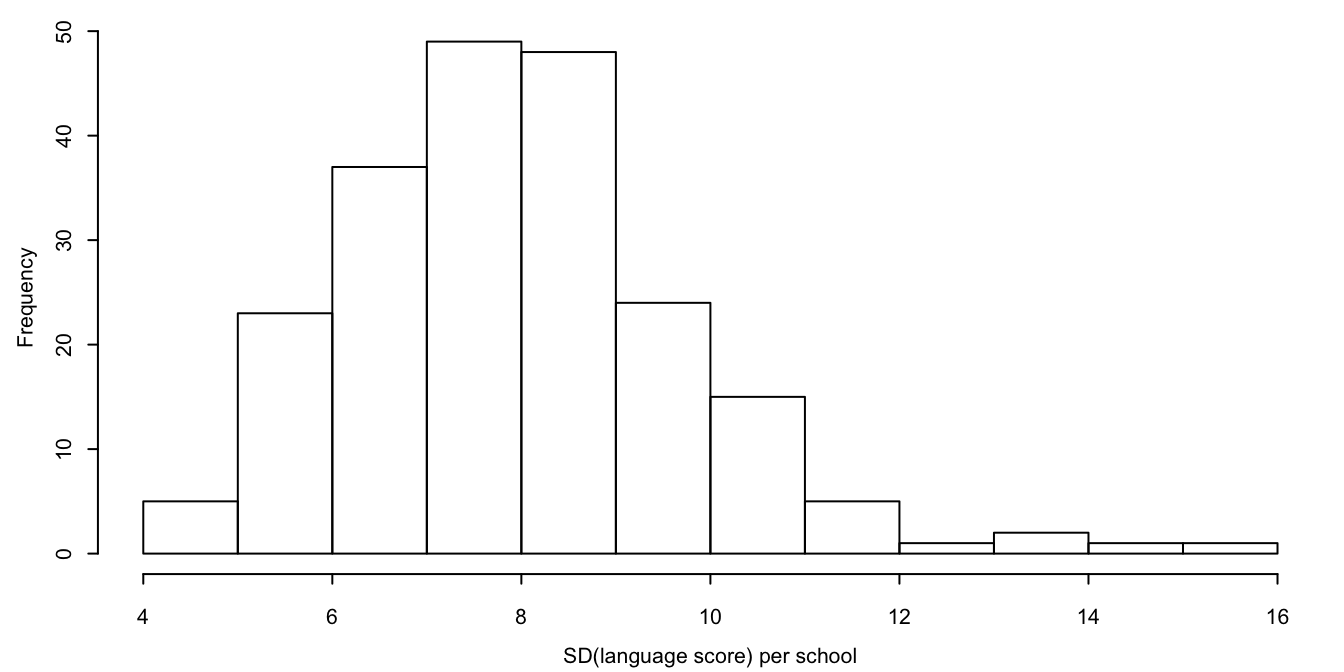
Figure 7.1: Distribution of standard deviations of language score per school.

The 2l.pan and 2l.norm methods are the oldest multilevel methods. Method 2l.pan is very fast, while method 2l.norm is more flexible since the within-cluster error variances may differ. To see which of these methods should be preferred for these data, let us study the distribution of the standard deviation of lpo by schools. Figure 7.1 shows that the standard deviation per school varies between 4 and 16, a fairly large spread. This suggests that 2l.norm might be preferred here.

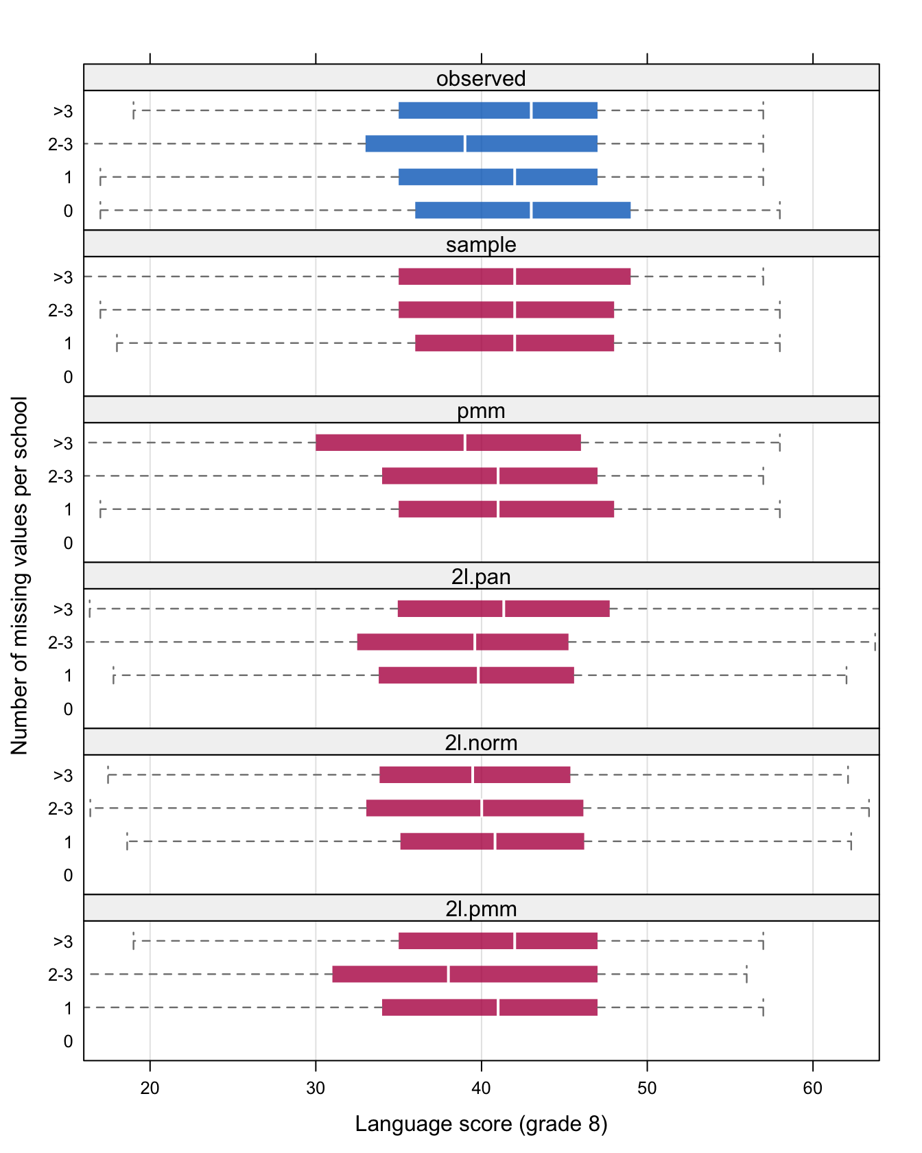
Box plots comparing the distribution of the observed data (blue), and the imputed data (red) under five methods, split according to the number of missing values per school.

Figure 7.2: Box plots comparing the distribution of the observed data (blue), and the imputed data (red) under five methods, split according to the number of missing values per school.

Figure 7.2 shows the box plot of the observed data (in blue) and the imputed data (in red) under each of the methods. Box plots are drawn for school with zero missing values, one missing value, two or three missing values and more than three missing values. Pupils in schools with one to three missing values have lower scores than pupils from a school with complete data. Pupils from schools with more than three missing values score similar to pupils from schools with complete data. It is interesting to study how well the different imputation methods preserve this feature in the data.

Method sample does not use any school information, and hence the imputations in all schools look alike. Methods pmm, 2l.pan, 2l.norm and 2l.pmm preserve the pattern, though the differences are less outspoken than in the observed data. Note that the distribution of the two normal methods (2l.pan and 2l.norm) have tails that extend beyond the range of the observed data (the maximum is 58). Hence, complete-data estimators based on the tails (e.g., finding the Top 10 Dutch schools) can be distorted by this use of the normal imputation.

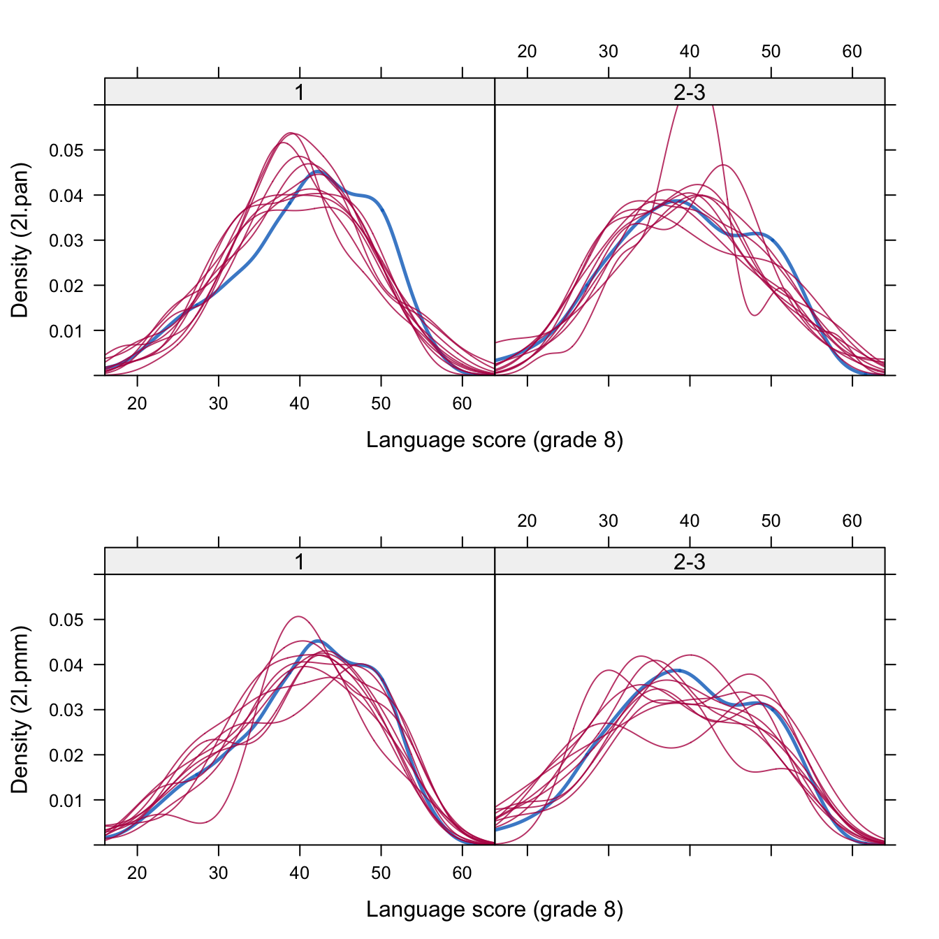
Figure 7.3: Density plots for schools with one and with two or three missing values for 2l.pan (top) and 2l.pmm (bottom).

Figure 7.3 shows the density plot of the 10 sets of imputed values (red) compared with the density plot of the observed values (blue). The top row corresponds to the 2l.pan method, and shows that some parts of the blue curve are not well represented by the imputed values. The method at the bottom row (2l.pmm) tracks the observed data distribution a little better.

Most research to date has concentrated on multilevel imputation using the normal model. In reality, normality is always an approximation, and it depends on the substantive question of how good this approximation should be. Two-level predictive mean matching is a promising alternative that can impute close to the data.