9.2 Sensitivity analysis
The imputations created in Section 9.1 are based on the assumption that the data are MAR (cf. Sections 1.2 and 2.2.4). While this is often a good starting assumption, it may not be realistic for the data at hand. When the data are not MAR, we can follow two strategies to obtain plausible imputations. The first strategy is to make the data “more MAR.” In particular, this strategy requires us to identify additional information that explains differences in the probability to be missing. This information is then used to generate imputations conditional on that information. The second strategy is to perform a sensitivity analysis. The goal of the sensitivity analysis is to explore the result of the analysis under alternative scenarios for the missing data. See Section 6.2 for a more elaborate discussion of these strategies.
This section explores sensitivity analysis for the Leiden 85+ Cohort data. In sensitivity analysis, imputations are generated according to one or more scenarios. The number of possible scenarios is infinite, but these are not equally likely. A scenario could be very simple, like assuming that everyone with a missing value had scored a “yes,” or assuming that those with missing blood pressures have the minimum possible value. While easy to interpret, such extreme scenarios are highly unlikely. Preferably, we should attempt to make an educated guess about both the direction and the magnitude of the missing data had they been observed. By definition, this guess needs to be based on external information beyond the data.
9.2.1 Causes and consequences of missing data
We continue with the Leiden 85+ Cohort data described in Section 9.1. The objective is to estimate the effect of blood pressure (BP) on mortality. BP was not measured for 126 individuals (121 systolic, 126 diastolic).
Attaching package: 'survival'The following object is masked from 'package:rpart':
solder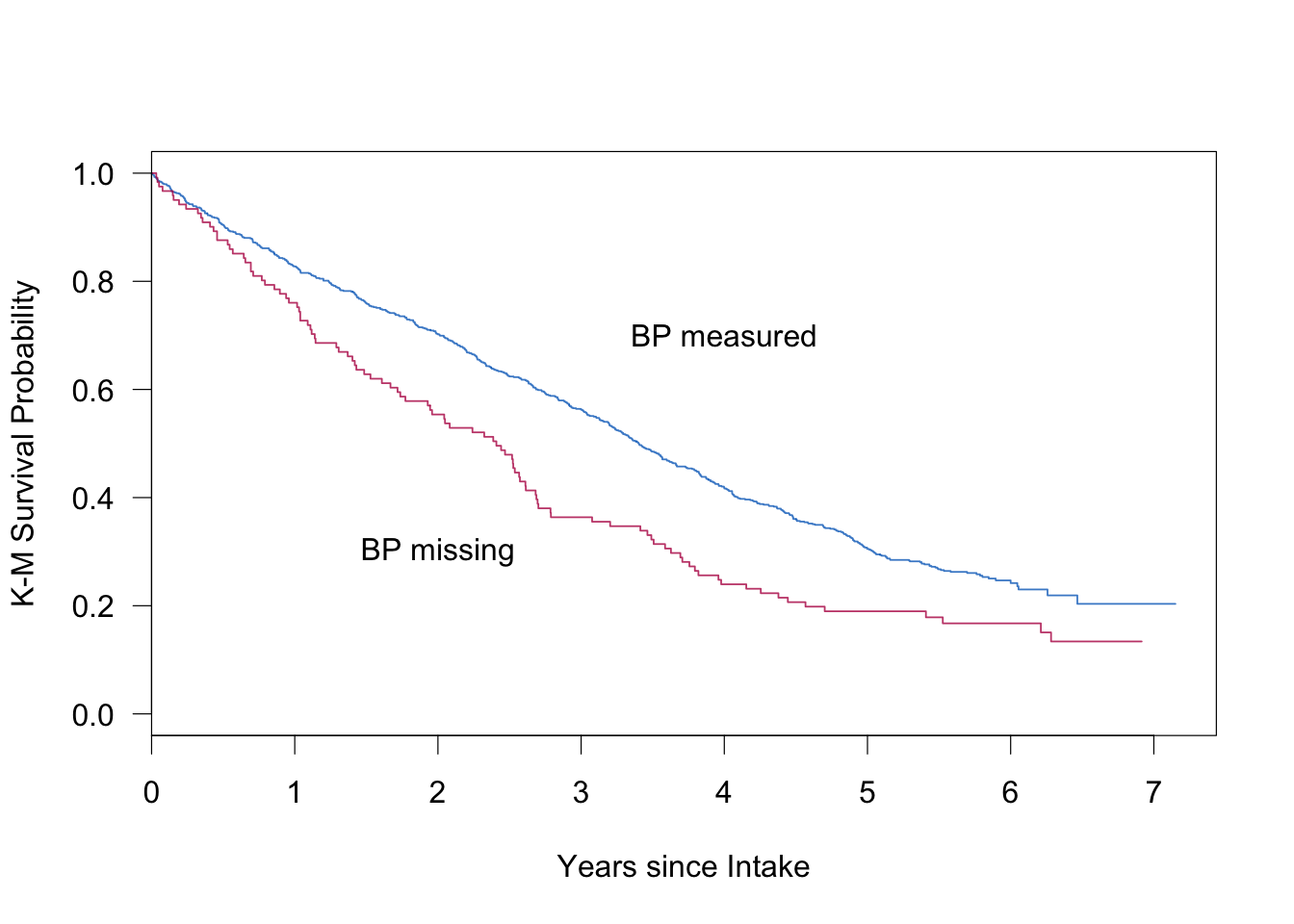
Figure 9.3: Kaplan–Meier curves of the Leiden 85+ Cohort, stratified according to missingness. The figure shows the survival probability since intake for the group with observed BP measures (blue) and the group with missing BP measures (red).
The missingness is strongly related to survival. Figure 9.3 displays the Kaplan-Meier survival curves for those with (\(n=835\)) and without (\(n=121\)) a measurement of systolic BP (SBP). BP measurement was missing for a variety of reasons. Sometimes there was a time constraint. In other cases the investigator did not want to place an additional burden on the respondent. Some subjects were too ill to be measured.
| Variable | Observed BP | Missing BP | |
|---|---|---|---|
| Age (year) | \(p<0.0001\) | ||
| 85–89 | 63 | 48 | |
| 90–94 | 32 | 34 | |
| 95+ | 6 | 18 | |
| Type of residence | \(p<0.0001\) | ||
| Independent | 52 | 35 | |
| Home for elderly | 35 | 54 | |
| Nursing home | 13 | 12 | |
| Activities of daily living (ADL) | \(p<0.001\) | ||
| Independent | 73 | 54 | |
| Dependent on help | 27 | 46 | |
| History of hypertension | \(p=0.06\) | ||
| No | 77 | 85 | |
| Yes | 23 | 15 |
Table 9.2 indicates that BP was measured less frequently for very old persons and for persons with health problems. Also, BP was measured more often if the BP was too high, for example if the respondent indicated a previous diagnosis of hypertension, or if the respondent used any medication against hypertension. The missing data rate of BP also varied during the period of data collection. The rate gradually increases during the first seven months of the sampling period from 5 to 40 percent of the cases, and then suddenly drops to a fairly constant level of 10–15 percent. A complicating factor here is that the sequence in which the respondents were interviewed was not random. High-risk groups, that is, elderly in hospitals and nursing homes and those over 95, were visited first.
| Survived | Hypertension: No | Hypertension: Yes |
|---|---|---|
| Yes | 8.7% (34/390) | 8.1% (10/124) |
| No | 19.2% (69/360) | 9.8% (8/82) |
Table 9.3 contains the proportion of persons for which BP was not measured, cross-classified by three-year survival and history of hypertension as measured during anamnesis. Of all persons who die within three years and that have no history of hypertension, more than 19% have no BP score. The rate for other categories is about 9%. This suggests that a relatively large group of individuals without hypertension and with high mortality risk is missing from the sample for which BP is known.
Using only the complete cases could lead to confounding by selection. The complete-case analysis might underestimate the mortality of the lower and normal BP groups, thereby yielding a distorted impression of the influence of BP on survival. This reasoning is somewhat tentative as it relies on the use of hypertension history as a proxy for BP. If true, however, we would expect more missing data from the lower BP measures. It is known that BP and mortality are inversely related in this age group, that is, lower BP is associated with higher mortality. If there are more missing data for those with low BP and high mortality (as in Table 9.3), selection of the complete cases could blur the effect of BP on mortality.
9.2.2 Scenarios
The previous section presented evidence that there might be more missing data for the lower blood pressures. Imputing the data under MAR can only account for nonresponse that is related to the observed data. However, the missing data may also be caused by factors that have not been observed. In order to study the influence of such factors on the final inferences, let us conduct a sensitivity analysis.
Section 3.8 advocated the use of simple adjustments to the imputed data as a way to perform sensitivity analysis. Table 3.6 lists possible values for an offset \(\delta\), together with an interpretation whether the value would be (too) small or (too) large. The next section uses the following range for \(\delta\): 0 mmHg (MCAR, too small), -5 mmHg (small), -10 mmHg (large), -15 mmHg (extreme) and -20 mmHg (too extreme). The last value is unrealistically low, and is primarily included to study the stability of the analysis in the extreme.
9.2.3 Generating imputations under the \(\delta\)-adjustment
Subtracting a fixed amount from the imputed values is easily achieved by the post processing facility in mice(). The following code first imputes under \(\delta = 0\)mmHg (MAR), then under \(\delta\) = -5 mmHg, and so on.
delta <- c(0, -5, -10, -15, -20)
post <- imp.qp$post
imp.all.undamped <- vector("list", length(delta))

for (i in 1:length(delta)) {
  d <- delta[i]
  cmd <- paste("imp[[j]][,i] <- imp[[j]][,i] +", d)
  post["rrsyst"] <- cmd
  imp <- mice(data2, pred = pred, post = post, maxit = 10,
              seed = i * 22)
  imp.all.undamped[[i]] <- imp
}
Note that we specify an adjustment in SBP only. Since imputed SBP is used to impute other incomplete variables, \(\delta\) will also affect the imputations in those. The strength of the effect depends on the correlation between SBP and the variable. Thus, using a \(\delta\)-adjustment for just one variable will affect many.
| \(\delta\) | Difference |
|---|---|
| 0 | -8.2 |
| -5 | -12.3 |
| -10 | -20.7 |
| -15 | -26.1 |
| -20 | -31.5 |
The mean of the observed systolic blood pressures is equal to 152.9 mmHg. Table 9.4 provides the differences in means between the imputed and observed data as a function of \(\delta\). For \(\delta\) = 0, i.e., under MAR, we find that the imputations are on average 8.2 mmHg lower than the observed blood pressure, which is in line with the expectations. As intended, the gap between observed and imputed increases as \(\delta\) decreases.
Note that for \(\delta\) = -10 mmHg, the magnitude of the difference with the MAR case (-20.7 + 8.2 = -12.5 mmHg) is somewhat larger in size than \(\delta\). The same holds for \(\delta\) = -15 mmHg and \(\delta\) = -20 mmHg. This is due to feedback of the \(\delta\)-adjustment itself via third variables. It is possible to correct for this, for example by multiplying \(\delta\) by a damping factor \(\sqrt{1-r^2}\), with \(r^2\) the proportion of explained variance of the imputation model for SBP. In R this can be done by changing the expression for cmd as
cmd <- paste("fit <- lm(y ~ as.matrix(x));
              damp <- sqrt(1 - summary(fit)$r.squared);
              imp[[j]][, i] <- imp[[j]][, i] + damp * ", d)
As the estimates of the complete-data model turned out to be very similar to the “raw” \(\delta\), this route is not further explored.
9.2.4 Complete-data model
The complete-data model is a Cox regression with survival since intake as the outcome, and with blood pressure groups as the main explanatory variable. The analysis is stratified by sex and age group. The preliminary data transformations needed for this analysis were performed as follows:
cda <- expression(
    sbpgp <- cut(rrsyst, breaks = c(50, 124, 144, 164, 184, 200,
                                    500)),
    agegp <- cut(lftanam, breaks = c(85, 90, 95, 110)),
    dead  <- 1 - dwa,
    coxph(Surv(survda, dead)
          ~ C(sbpgp, contr.treatment(6, base = 3))
          + strata(sexe, agegp)))
imp <- imp.all.damped[[1]]
fit <- with(imp, cda)
The cda object is an expression vector containing several statements needed for the complete-data model. The cda object will be evaluated within the environment of the imputed data, so (imputed) variables like rrsyst and survda are available during execution. Derived variables like sbpgp and agegp are temporary and disappear automatically. When evaluated, the expression vector returns the value of the last expression, in this case the object produced by coxph(). The expression vector provides a flexible way to apply R code to the imputed data. Do not forget to include commas to separate the individual expressions. The pooled hazard ratio per SBP group can be calculated by
as.vector(exp(summary(pool(fit))[, 1]))Warning: Unknown or uninitialised column: 'df.residual'.Warning in pool.fitlist(getfit(object), dfcom = dfcom): Large
sample assumed.[1] 1.758 1.433 1.065 1.108 0.861| \(\delta\) | < 125 mmHg | 125-140 mmHg | > 200 mmHG |
|---|---|---|---|
| 0 | 1.76 (1.36–2.28) | 1.43 (1.16–1.77) | 0.86 (0.44–1.67) |
| -5 | 1.81 (1.42–2.30) | 1.45 (1.18–1.79) | 0.88 (0.50–1.55) |
| -10 | 1.89 (1.47–2.44) | 1.50 (1.21–1.86) | 0.90 (0.51–1.59) |
| -15 | 1.82 (1.39–2.40) | 1.45 (1.14–1.83) | 0.88 (0.49–1.57) |
| -20 | 1.80 (1.39–2.35) | 1.46 (1.17–1.83) | 0.85 (0.48–1.50) |
| CCA | 1.76 (1.36–2.28) | 1.48 (1.19–1.84) | 0.89 (0.51–1.57) |
Table 9.5 provides the hazard ratio estimates under the different scenarios for three SBP groups. A risk ratio of 1.76 means that the mortality risk (after correction for sex and age) in the group “< 125mmHg” is 1.76 times the risk of the reference group “145-160mmHg.” The inverse relation relation between mortality and blood pressure in this age group is consistent, where even the group with the highest blood pressures have (nonsignificant) lower risks.
Though the imputations differ dramatically under the various scenarios, the hazard ratio estimates for different \(\delta\) are close. Thus, the results are essentially the same under all specified MNAR mechanisms. Also observe that the results are close to those from the analysis of the complete cases.
9.2.5 Conclusion
Sensitivity analysis is an important tool for investigating the plausibility of the MAR assumption. This section explored the use of an informal, simple and direct method to create imputations under nonignorable models by simply deducting some amount from the imputations.
Section 3.8.1 discussed shift, scale and shape parameters for nonignorable models. We only used a shift parameter here, which suited our purposes in the light of what we knew about the causes of the missing data. In other applications, scale or shape parameters could be more natural. The calculations are easily adapted to such cases.