3.4 Predictive mean matching
3.4.1 Overview
Predictive mean matching calculates the predicted value of target variable \(Y\) according to the specified imputation model. For each missing entry, the method forms a small set of candidate donors (typically with 3, 5 or 10 members) from all complete cases that have predicted values closest to the predicted value for the missing entry. One donor is randomly drawn from the candidates, and the observed value of the donor is taken to replace the missing value. The assumption is the distribution of the missing cell is the same as the observed data of the candidate donors.
Predictive mean matching is an easy-to-use and versatile method. It is fairly robust to transformations of the target variable, so imputing \(\log(Y)\) often yields results similar to imputing \(\exp(Y)\). The method also allows for discrete target variables. Imputations are based on values observed elsewhere, so they are realistic. Imputations outside the observed data range will not occur, thus evading problems with meaningless imputations (e.g., negative body height). The model is implicit (Little and Rubin 2002), which means that there is no need to define an explicit model for the distribution of the missing values. Because of this, predictive mean matching is less vulnerable to model misspecification than the methods discussed in Sections 3.2 and 3.3.
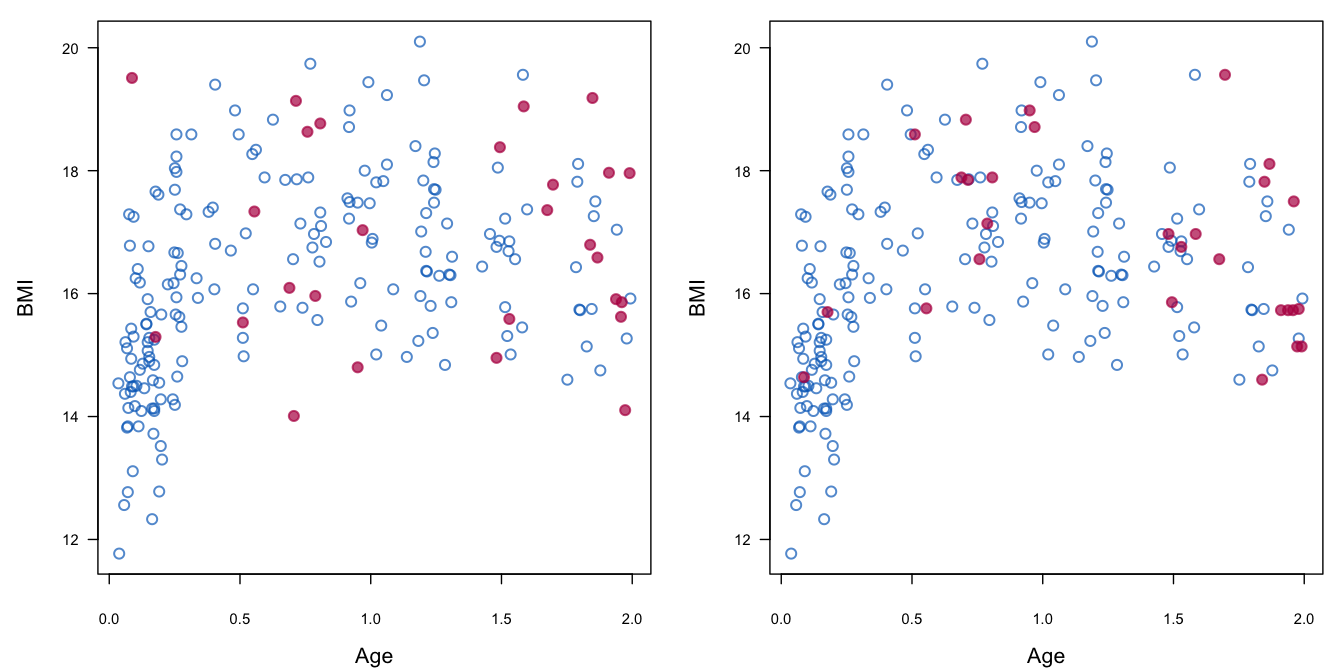
Figure 3.6: Robustness of predictive mean matching (right) relative to imputation under the linear normal model (left).
Figure 3.6 illustrates the robustness of predictive mean matching relative to the normal model. The figure displays the body mass index (BMI) of children aged 0–2 years. BMI rapidly increases during the first half year of life, has a peak around 1 year and then slowly drops at ages when the children start to walk. The imputation model is, however, incorrectly specified, being linear in age. Imputations created under the normal model display in an incorrect slowly rising pattern, and contain several implausible values. In contrast, the imputations created by predictive mean matching follow the data quite nicely, even though the predictive mean itself is clearly off-target for some of the ages. This example shows that predictive mean matching is robust against misspecification, where the normal model is not.
Predictive mean matching is an example of a hot deck method, where values are imputed using values from the complete cases matched with respect to some metric. The expression “hot deck” literally refers to a pack of computer control cards containing the data of the cases that are in some sense close. Reviews of hot deck methods can be found in Ford (1983), Brick and Kalton (1996), Koller-Meinfelder (2009), Andridge and Little (2010) and De Waal, Pannekoek, and Scholtus (2011, 249–55, 349–55).
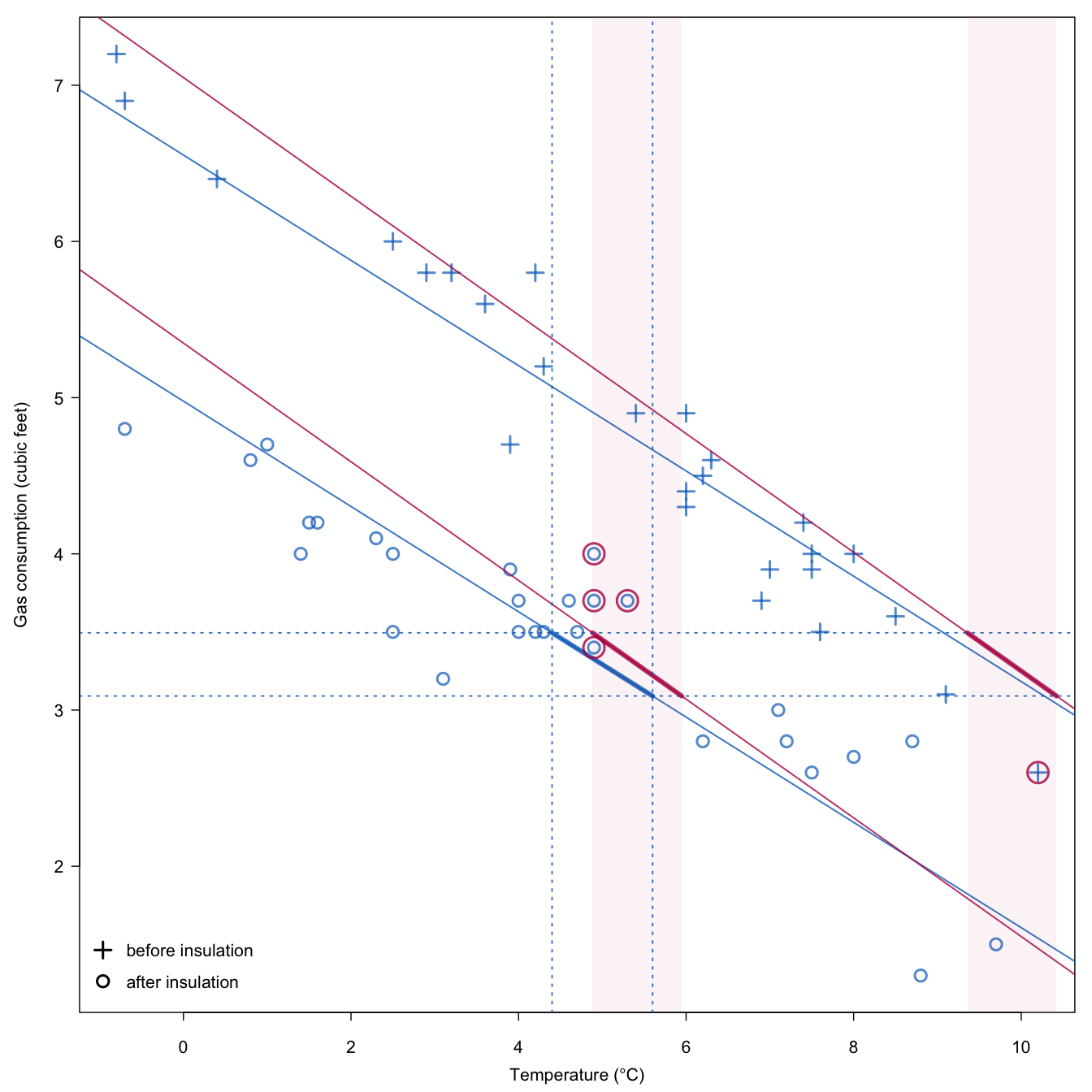
Figure 3.7: Selection of candidate donors in predictive mean matching with the stochastic matching distance.
Figure 3.7 is an illustration of the method using the whiteside data. The predictor is equal to 5\(^\circ\mathrm{C}\) and the bandwidth is 1.2. The thick blue line indicates the area of the target variable where matches should be sought. The blue part of the figure are considered fixed. The red line correspond to one random draw of the line parameters to incorporate sampling uncertainty. The two light-red bands indicate the area where matches are permitted. In this particular instance, five candidate donors are found, four from the subgroup “after insulation” and one from the subgroup “before insulation.” The last step is to make a random draw among these five candidates. The red parts in the figure will vary between different imputed datasets, and thus the set of candidates will also vary over the imputed datasets.
The data point at coordinate (10.2, 2.6) is one of the candidate donors. This point differs from the incomplete unit in both temperature and insulation status, yet it is selected as a candidate donor. The advantage of including the point is that closer matches in terms of the predicted values are possible. Under the assumption that the distribution of the target in different bands is similar, including points from different bands is likely to be beneficial.
3.4.2 Computational details\(^\spadesuit\)
Various metrics are possible to define the distance between the cases. The predictive mean matching metric was proposed by Rubin (1986) and Little (1988). This metric is particularly useful for missing data applications because it is optimized for each target variable separately. The predicted value only needs to be a convenient one-number summary of the important information that relates the covariates to the target. Calculation is straightforward, and it is easy to include nominal and ordinal variables.
Once the metric has been defined, there are various ways to select the donor. Let \(\hat y_i\) denote the predicted value of the rows with an observed \(y_i\) where \(i=1,\dots,n_1\). Likewise, let \(\hat y_j\) denote the predicted value of the rows with missing \(y_j\) where \(j=1,\dots,n_0\). Andridge and Little (2010) distinguish four methods:
Choose a threshold \(\eta\), and take all \(i\) for which \(|\hat y_i-\hat y_j|<\eta\) as candidate donors for imputing \(j\). Randomly sample one donor from the candidates, and take its \(y_i\) as replacement value.
Take the closest candidate, i.e., the case \(i\) for which \(|\hat y_i-\hat y_j|\) is minimal as the donor. This is known as “nearest neighbor hot deck,” “deterministic hot deck” or “closest predictor.”
Find the \(d\) candidates for which \(|\hat y_i-\hat y_j|\) is minimal, and sample one of them. Usual values for \(d\) are 3, 5 and 10. There is also an adaptive method to specify the number of donors (Schenker and Taylor 1996).
Sample one donor with a probability that depends on \(|\hat y_i-\hat y_j|\) (Siddique and Belin 2008).
In addition, it is useful to distinguish four types of matching:
Type 0: \(\hat y=X_\mathrm{obs}\hat\beta\) is matched to \(\hat y_j=X_\mathrm{mis}\hat\beta\);
Type 1: \(\hat y=X_\mathrm{obs}\hat\beta\) is matched to \(\dot y_j=X_\mathrm{mis}\dot\beta\);
Type 2: \(\dot y=X_\mathrm{obs}\dot\beta\) is matched to \(\dot y_j=X_\mathrm{mis}\dot\beta\);
Type 3: \(\dot y=X_\mathrm{obs}\dot\beta\) is matched to \(\ddot y_j=X_\mathrm{mis}\ddot\beta\).
Here \(\hat\beta\) is the estimate of \(\beta\), while \(\dot\beta\) is a value randomly drawn from the posterior distribution of \(\beta\). Type 0 matching ignores the sampling variability in \(\hat\beta\), leading to improper imputations. Type 2 matching appears to solve this. However, it is insensitive to the process of taking random draws of \(\beta\) if there are only a few variables. In the extreme case, with a single \(X\), the set of candidate donors based on \(|\dot y_i-\dot y_j|\) remains unchanged under different values of \(\dot\beta\), so the same donor(s) get selected too often. Type 1 matching is a small but nifty adaptation of the matching distance that seems to alleviate the problem. The difference with Type 0 and Type 2 matching is that in Type 1 matching only \(X_\mathrm{mis}\dot\beta\) varies stochastically and does not cancel out any more. As a result \(\dot\eta\) incorporates between-imputation variation. Type 3 matching creates two draws for \(\beta\), one for the donor set and one for the recipient set. In retrospect, it is interesting to note that Type 1 matching was already described by Little (1988 eq. 4). It disappeared from the literature, only to reappear two decades later in the works of Koller-Meinfelder (2009, 43) and White, Royston, and Wood (2011, 383).
Algorithm 3.3 (Predictive mean matching with a Bayesian \(\beta\) and a stochastic matching distance (Type~1 matching).)
Calculate \(\dot\beta\) and \(\hat\beta\) by Steps 1-8 of Algorithm 3.1.
Calculate \(\dot\eta(i,j)=|X_i^\mathrm{obs}\hat\beta-X_j^\mathrm{mis}\dot\beta|\) with \(i=1,\dots,n_1\) and \(j=1,\dots,n_0\).
Construct \(n_0\) sets \(Z_j\), each containing \(d\) candidate donors, from \(Y_\mathrm{obs}\) such that \(\sum_d\dot\eta(i,j)\) is minimum for all \(j=1,\dots,n_0\). Break ties randomly.
Draw one donor \(i_j\) from \(Z_j\) randomly for \(j=1,\dots,n_0\).
- Calculate imputations \(\dot y_j = y_{i_j}\) for \(j=1,\dots,n_0\).
Algorithm 3.3 provides the steps used in predictive mean matching using Bayesian parameter draws for \(\beta\). It is possible to create the bootstrap version of this algorithm that will also evade the need to draw \(\beta\) along the same lines as Algorithm 3.2. Given that the number of candidate donors and the model for the mean is provided by the user, the algorithm does not need an explicit specification of the distribution.
Morris, White, and Royston (2014) suggested a variation called local residuals draws. Rather than taking the observed value of the donor, this method borrows the residual from the donor, and adds that to the predicted value from the target case. Thus, imputations are not equal to observed values, and can extend beyond the range of the observed data. This may address concerns about variability of imputations.
3.4.3 Number of donors
There are different strategies for defining the set and number of candidate donors. Setting \(d = 1\) is generally considered to be too low, as it may reselect the same donor over and over again. Predictive mean matching performs very badly when \(d\) is small and there are lots of ties for the predictors among the individuals to be imputed. The reason is that the tied individuals all get the same imputed value in each imputed dataset when \(d = 1\) (Ian White, personal communication). Setting \(d\) to a high value (say \(n/10\)) alleviates the duplication problem, but may introduce bias since the likelihood of bad matches increases. Schenker and Taylor (1996) evaluated \(d = 3\), \(d = 10\) and an adaptive scheme. The adaptive method was slightly better than using a fixed number of candidates, but the differences were small. compared various settings for \(d\), and found that \(d = 5\) and \(d = 10\) generally provided the best results. found that \(d = 5\) may be too high for sample size lower than \(n = 100\), and suggested setting \(d = 1\) for better point estimates for small samples. Gaffert, Koller-Meinfelder, and Bosch (2016) explored scenarios in which candidate donors have different probabilities to be drawn, where the probability depends on the distance between the donor and recipient cases. As all observed cases can be donors in this scenario, there is no need to specify \(d\). Instead a closeness parameter needs to be specified, and this was made adaptive to the data. An advantage of using all donors is that the variance of the imputations can be corrected by the Parzen correction, which alleviates concerns about insufficient variability of the imputes. Their simulations showed that with a small sample (\(n = 10\)), the adaptive method is clearly superior to methods with a fixed donor pool. The method is available in mice as the midastouch method. There is also a separate midastouch package in R. Related work can be found in Tutz and Ramzan (2015).
The default in mice is \(d = 5\), and represents a compromise. The above results suggest that an adaptive method for setting \(d\) could improve small sample behavior. Meanwhile, the number of donors can be changed through the donors argument.
| Method | Bias | % Bias | Coverage | CI Width | RMSE | |
|---|---|---|---|---|---|---|
| Missing \(y\), \(n = 50\) | \(d\) | |||||
pmm |
1 | 0.016 | 5.4 | 0.884 | 0.252 | 0.071 |
pmm |
3 | 0.028 | 9.7 | 0.890 | 0.242 | 0.070 |
pmm |
5 | 0.039 | 13.6 | 0.876 | 0.241 | 0.075 |
pmm |
10 | 0.065 | 22.4 | 0.806 | 0.245 | 0.089 |
| Missing \(x\) | ||||||
pmm |
1 | -0.002 | 0.8 | 0.916 | 0.223 | 0.063 |
pmm |
3 | 0.002 | 0.9 | 0.931 | 0.228 | 0.061 |
pmm |
5 | 0.008 | 2.8 | 0.938 | 0.237 | 0.062 |
pmm |
10 | 0.028 | 9.6 | 0.946 | 0.261 | 0.067 |
| Listwise deletion | 0.000 | 0.0 | 0.946 | 0.251 | 0.063 | |
| Missing \(y\), \(n = 50\) | \(\kappa\) | |||||
midastouch |
auto | 0.013 | 4.5 | 0.920 | 0.265 | 0.066 |
midastouch |
2 | 0.032 | 11.1 | 0.917 | 0.273 | 0.068 |
midastouch |
3 | 0.018 | 6.2 | 0.927 | 0.261 | 0.064 |
midastouch |
4 | 0.012 | 4.1 | 0.926 | 0.260 | 0.064 |
| Missing \(x\) | ||||||
midastouch |
auto | -0.003 | 0.9 | 0.932 | 0.241 | 0.060 |
midastouch |
2 | 0.013 | 4.4 | 0.959 | 0.264 | 0.059 |
midastouch |
3 | 0.000 | 0.2 | 0.947 | 0.245 | 0.058 |
midastouch |
4 | -0.004 | 1.4 | 0.940 | 0.237 | 0.058 |
| Listwise deletion | 0.000 | 0.0 | 0.946 | 0.251 | 0.063 | |
| Missing \(y\), \(n = 1000\) | \(d\) | |||||
pmm |
1 | 0.001 | 0.2 | 0.929 | 0.056 | 0.014 |
pmm |
3 | 0.001 | 0.4 | 0.950 | 0.056 | 0.013 |
pmm |
5 | 0.002 | 0.6 | 0.951 | 0.055 | 0.013 |
pmm |
10 | 0.003 | 1.2 | 0.932 | 0.054 | 0.013 |
| Missing \(x\) | ||||||
pmm |
1 | 0.000 | 0.2 | 0.926 | 0.041 | 0.011 |
pmm |
3 | 0.000 | 0.1 | 0.933 | 0.041 | 0.011 |
pmm |
5 | 0.000 | 0.1 | 0.937 | 0.042 | 0.011 |
pmm |
10 | 0.000 | 0.1 | 0.928 | 0.042 | 0.011 |
| Listwise deletion | 0.000 | 0.1 | 0.955 | 0.050 | 0.012 |
Table 3.3 repeats the simulation experiment done in Tables 3.1 and 3.2 for predictive mean matching for three different choices of the number \(d\) of candidate donors. Results are given for \(n = 50\) and \(n = 1000\). For \(n = 50\) we find that \(\beta_1\) is increasingly biased towards the null for larger \(d\). Because of the bias, the coverage is lower than nominal. For missing \(x\) the bias is much smaller. Setting \(d\) to a lower value, as recommended by Kleinke (2017), improves point estimates, but the magnitude of the effect depends on whether the missing values occur in \(x\) or \(y\). For the sample size \(n = 1000\) predictive mean matching appears well calibrated for \(d = 5\) for missing data in \(y\), and has slight undercoverage for missing data in \(x\). Note that Table 3.3 in the first edition of this book presented incorrect information because it had erroneously imputed the data by norm instead of pmm.
3.4.4 Pitfalls
The obvious danger of predictive mean matching is the duplication of the same donor value many times. This problem is more likely to occur if the sample is small, or if there are many more missing data than observed data in a particular region of the predicted value. Such unbalanced regions are more likely if the proportion of incomplete cases is high, or if the imputation model contains variables that are very strongly related to the missingness. For small samples the donor pool size can be reduced, but be aware that this may not work if there are only a few predictors.
The traditional method does not work for a small number of predictors. Heitjan and Little (1991) report that for just two predictors the results were “disastrous.” The cause of the problem appears to be related to their use of Type 0 matching. The default in mice is Type 1 matching, which works better for small number of predictors. The setting can be changed to Type 0 or Type 2 matching through the matchtype argument.
Predictive mean matching is no substitute for sloppy modeling. If the imputation model is misspecified, performance can become poor if there are strong relations in the data that are not modeled (Morris, White, and Royston 2014). The default imputation model in mice consists of a linear main effect model conditional on all other variables, but this may be inadequate in the presence of strong nonlinear relations. More generally, any terms appearing in the complete-data model need to be accounted for in the imputation model. Morris, White, and Royston (2014) advise to spend efforts on specifying the imputation model correctly, rather than expecting predictive mean matching to do the work.
3.4.5 Conclusion
Predictive mean matching with \(d = 5\) is the default in mice() for continuous data. The method is robust against misspecification of the imputation model, yet performs as well as theoretically superior methods. In the context of missing covariate data, Marshall, Altman, and Holder (2010) concluded that predictive mean matching “produced the least biased estimates and better model performance measures.” Another simulation study that addressed skewed data concluded that predictive mean matching “may be the preferred approach provided that less than 50% of the cases have missing data and the missing data are not MNAR” (Marshall et al. 2010). Kleinke (2017) found that the method works well across a wide variety of scenarios, but warned the default cannot address severe skewness or small samples.
The method works best with large samples, and provides imputations that possess many characteristics of the complete data. Predictive mean matching cannot be used to extrapolate beyond the range of the data, or to interpolate within the range of the data if the data at the interior are sparse. Also, it may not perform well with small datasets. Bearing these points in mind, predictive mean matching is a great all-around method with exceptional properties.