9.3 Correct prevalence estimates from self-reported data

9.3.1 Description of the problem

Prevalence estimates for overweight and obesity are preferably based on standardized measured data of height and weight. However, obtaining such measures is logistically challenging and costly. An alternative is to ask persons to report their own height and weight. It is well known that such measures are subject to systematic biases. People tend to overestimate their height and underestimate their weight. A recent overview covering 64 studies can be found in Gorber et al. (2007).

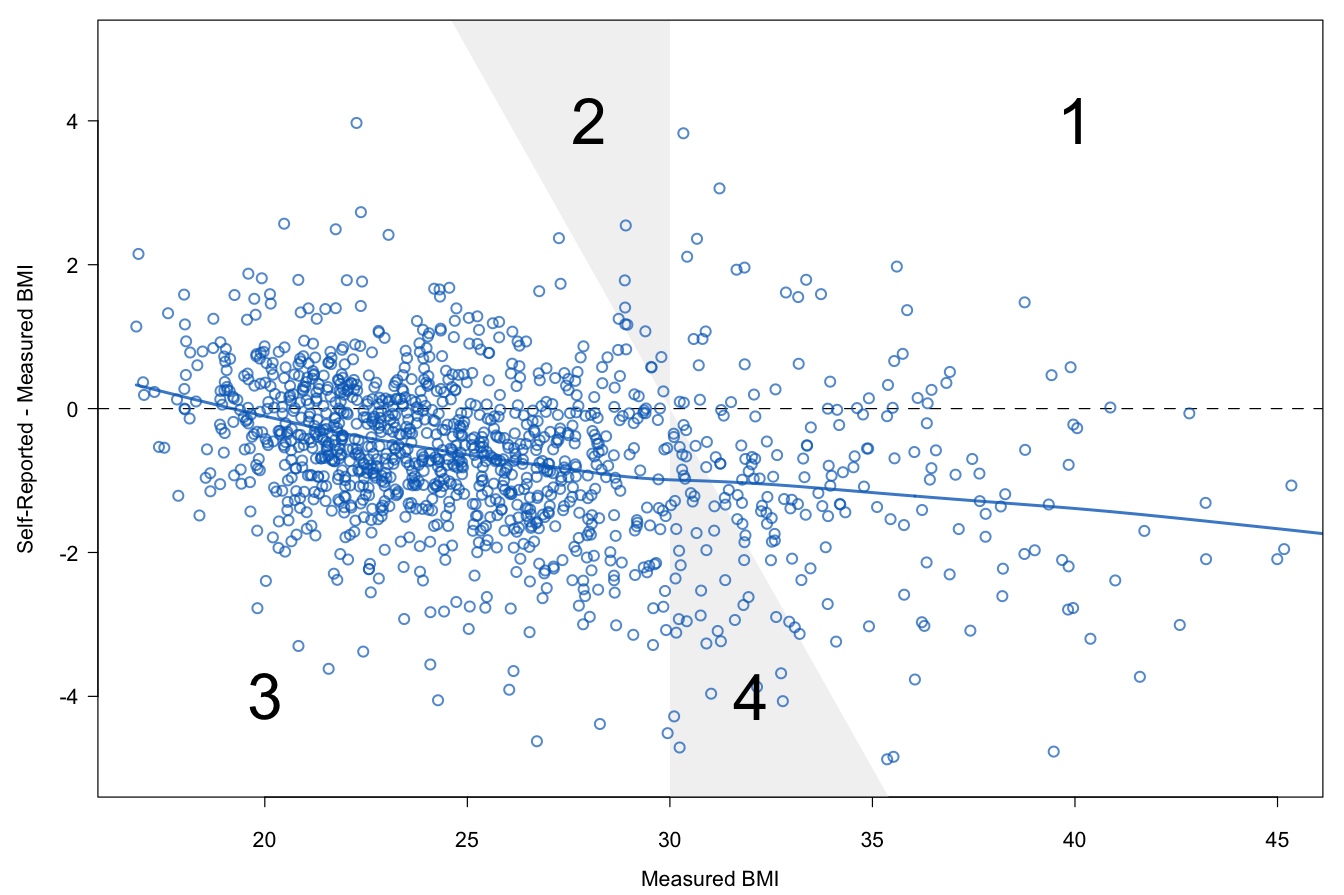
Figure 9.4: Underestimation of obesity prevalence in self-reported data. Self-reported BMI is on average 1–2\(\mathrm{kg}/\mathrm{m}^2\) too low. Lines are fitted by LOWESS.

Body Mass Index (BMI) is calculated from height and weight as \(\mathrm{kg}/\mathrm{m}^2\). For BMI both biases operate in the same direction, so any self-reporting biases are amplified in BMI. Figure 9.4 is drawn from data of Krul, Daanen, and Choi (2010). Self-reported BMI is on average 1–2\(\mathrm{kg}/\mathrm{m}^2\) lower than measured BMI.

BMI values can be categorized into underweight (BMI \(<\) 18.5), normal (18.5 \(\leq\) BMI \(<\) 25), overweight (25 \(\leq\) BMI \(<\) 30), and obese (BMI \(\geq\) 30). Self-reported BMI may assign subjects to a category that is too low. In Figure 9.4 persons in the white area labeled “1” are obese according to both self-reported and measured BMI. Persons in the white area labeled “3” are non-obese. The shaded areas represent disagreement between measured and self-reported obesity. The shaded area “4” are obese according to measured BMI, but not to self-report. The reverse holds for the shaded area “2.” Due to self-reporting bias, the number of persons located in area “4” is generally larger than in area “2,” leading to underestimation. There have been many attempts to correct measured height and weight for bias using predictive equations. These attempts have generally not been successful. The estimated prevalences were often still found to be too low after correction. Moreover, there is substantial heterogeneity in the proposed predictive formulae, resulting in widely varying prevalence estimates. See Visscher et al. (2006) for a summary of these issues. The current consensus is that it is not possible to estimate overweight and obesity prevalence from self-reported data. Dauphinot et al. (2008) even suggested to lower cut-off values for obesity based on self-reported data.

The goal is to estimate obesity prevalence in the population from self-reported data. This estimate should be unbiased in the sense that, on average, it should be equal to the estimate that would have been obtained had data been truly measured. Moreover, the estimate must be accompanied by a standard error or a confidence interval.

9.3.2 Don’t count on predictions

Table 4 in Visscher et al. (2006) lists 36 predictive equations that have been proposed over the years. Visscher et al. (2006) observed that these equations predict too low. This section explains why this happens.

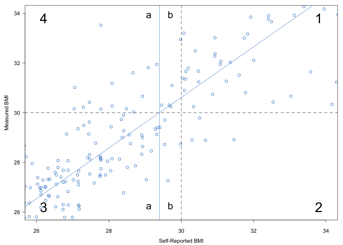
Figure 9.5: Illustration of the bias of predictive equations. In general, the combined region 2 + 3b will have fewer cases than region 4a. Thiscauses a downward bias in the prevalence estimate.

Figure 9.5 plots the data of Figure 9.4 in a different way. The figure is centered around the BMI of 30 \(\mathrm{kg}/\mathrm{m}^2\). The two dashed lines divide the area into four quadrants. Quadrant 1 contains the cases that are obese according to both BMI values. Quadrant 3 contains the cases that are classified as non-obese according to both. Quadrant 2 holds the subjects that are classified as obese according to self-report, but not according to measured BMI. Quadrant 4 has the opposite interpretation. The area and quadrant numbers used in Figures 9.4 and 9.5 correspond to identical subdivisions in the data.

The “true obese” in Figure 9.5 lie in quadrants 1 and 4. The obese according to self-report are located in quadrants 1 and 2. Observe that the number of cases in quadrant 2 is smaller than in quadrant 4, a result of the systematic bias that is observed in humans. Using uncorrected self-report thus leads to an underestimate of the true prevalence.

The regression line that predicts measured BMI from self-reported BMI is added to the display. This line intersects the horizontal line that separates quadrant 3 from quadrant 4 at a (self-reported) BMI value of 29.4 \(\mathrm{kg}/\mathrm{m}^2\). Note that using the regression line to predict obese versus non-obese is in fact equivalent to classifying all cases with a self-report of 29.4 \(\mathrm{kg}/\mathrm{m}^2\) or higher as obese. Thus, the use of the regression line as a predictive equation effectively shifts the vertical dashed line from 30 \(\mathrm{kg}/\mathrm{m}^2\) to 29.4 \(\mathrm{kg}/\mathrm{m}^2\). Now we can make the same type of comparison as before. We count the number of cases in quadrant 2 + section 3b (\(n_1\)), and compare it to the count in region 4a (\(n_2\)). The difference \(n_2-n_1\) is now much smaller, thanks to the correction by the predictive equation.

However, there is still bias remaining. This comes from the fact that the distribution on the left side is more dense. The number of subjects with a BMI of 28 \(\mathrm{kg}/\mathrm{m}^2\) is typically larger than the number of subjects with a BMI of 32 \(\mathrm{kg}/\mathrm{m}^2\). Thus, even if a symmetric normal distribution around the regression line is correct, \(n_2\) is on average larger than \(n_1\). This yields bias in the predictive equation.

Observe that this effect will be stronger if the regression line becomes more shallow, or equivalently, if the spread around the regression line increases. Both are manifestation of less-than-perfect predictability. Thus, predictive equations only work well if the predictability is very high, but they are systematically biased in general.

9.3.3 The main idea

Table 9.6: Basic variables needed to correct overweight/obesity prevalence for self-reporting. Note: The survey data are representative for the population of interest, possibly after correction for design factors.

Name	Description
age	Age (years)
sex	Sex (M/F)
hm	Height measured (cm)
hr	Height reported (cm)
wm	Weight measured (kg)
wr	Weight reported (kg)

Table 9.6 lists the six variable names needed in this application. Let us assume that we have two data sources available:

• The calibration dataset contains \(n_c\) subjects for which both self-reported and measured data are available;

• The survey dataset contains \(n_s\) subjects with only the self-reported data.

We assume that the common variables in these two datasets are comparable.

The idea is to stack the datasets, multiply impute the missing values for hm and wm in the survey data and estimate the overweight and obesity prevalence (and their standard errors) from the imputed survey data. See Schenker, Raghunathan, and Bondarenko (2010) for more background.

9.3.4 Data

The calibration sample is taken from Krul, Daanen, and Choi (2010). The dataset contains of \(n_c\) = 1257 Dutch subjects with both measured and self-reported data. The survey sample consists of \(n_s\) = 803 subjects of a representative sample of Dutch adults aged 18-75 years. These data were collected in November 2007 either online or using paper-and-pencil methods. The missing data pattern in the combined data is summarized as

data <- selfreport[, c("age", "sex", "hm", "hr", "wm", "wr")]
md.pattern(data, plot = FALSE)

     age sex hr wr  hm  wm     
1257   1   1  1  1   1   1    0
803    1   1  1  1   0   0    2
       0   0  0  0 803 803 1606

The row containing all ones corresponds to the 1257 observations from the calibration sample with complete data, whereas the rows with a zero on hm and wm correspond to 803 observations from the survey sample (where hm and wm were not measured).

We apply predictive mean matching (cf. Section 3.4) to impute hm and wm in the 803 records from the survey data. The number of imputations \(m=10\). The complete-data estimates are calculated on each imputed dataset and combined using Rubin’s pooling rules to obtain prevalence rates and the associated confidence intervals as in Sections 2.3.2 and 2.4.

9.3.5 Application

The mice() function can be used to create \(m=10\) multiply imputed datasets. We imputed measured height, measured weight and and measured BMI using the following code:

bmi <- function(h, w) w / (h / 100)^2
meth <- make.method(selfreport)
meth[c("prg", "edu", "etn")] <- ""
meth["bm"] <- "~ bmi(hm, wm)"
pred <- make.predictorMatrix(selfreport)
pred[, c("src", "id", "pop", "prg", "edu", "etn",
         "web", "bm", "br")] <- 0
imp <- mice(selfreport, pred = pred, meth = meth, m = 10,
            seed = 66573, maxit = 20, print = FALSE)

The code defines a bmi() function for use in passive imputation to calculate bmi. The predictor matrix is set up so that only age, sex, hr and wr are permitted to impute hm and wm.

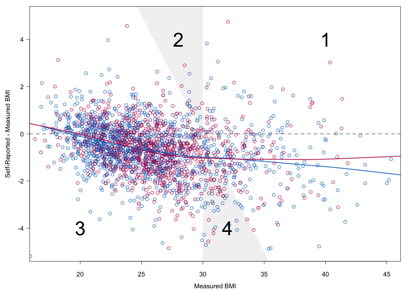
Figure 9.6: Relation between measured BMI and self-reported BMI in the calibration (blue) and survey (red) data in the first imputed dataset.

Figure 9.6 is a diagnostic plot to check whether the imputations maintain the relation between the measured and the self-reported data. The plot is identical to Figure 9.4, except that the imputed data from the survey data (in red) have been added. Imputations have been taken from the first imputed dataset. The figure shows that the red and blue dots are similar in terms of location and spread. Observe that BMI in the survey data is slightly higher. The very small difference between the smoothed lines across all measured BMI values confirms this notion. We conclude that the relation between self-reported and measured BMI as observed in the calibration data successfully “migrated” to the survey data.

Table 9.7: Obesity prevalence estimate (%) and standard error (se) in the survey data (\(n=803\)), reported (observed data) and corrected (imputed).

			Reported		Corrected
Sex	Age	\(n\)	%	se	%	se
Male	18-29	69	8.7	3.4	9.4	3.9
	30-39	73	11.0	3.7	15.7	5.0
	40-49	66	9.1	3.6	12.5	4.8
	50-59	91	20.9	4.3	25.4	5.2
	60-75	101	7.9	2.7	15.6	4.2
	18-75	400	11.7	1.6	16.0	2.0
Female	18-29	68	14.7	4.3	16.3	5.7
	30-39	69	26.1	5.3	28.4	6.6
	40-49	68	19.1	4.8	25.4	6.1
	50-59	81	25.9	4.9	32.8	6.0
	60-75	117	11.1	2.9	17.1	4.6
	18-75	403	18.6	1.9	23.0	2.4
All	18-75	803	15.2	1.3	19.5	1.5

Table 9.7 contains the prevalence estimates based on the survey data given for self-report and corrected for self-reporting bias. The estimates themselves are variable and have large standard errors. It is easy to infer that the size of the correction depends on age. Note that the standard errors of the corrected estimates are always larger than for the self-report. This reflects the information lost due to the correction. To obtain an equally precise estimate, the sample size of the study with only self-reports needs to be larger than the sample size of the study with direct measures.

9.3.6 Conclusion

Predictive equations to correct for self-reporting bias will only work if the percentage of explained variance is very high. In the general case, they have a systematic downward bias, which makes them unsuitable as correction methods. The remedy is to explicitly account for the residual distribution. We have done so by applying multiple imputation to impute measured height and weight. In addition, multiple imputation produces the correct standard errors of the prevalence estimates.