4.5 Fully conditional specification

4.5.1 Overview

Fully conditional specification (FCS) imputes multivariate missing data on a variable-by-variable basis (Van Buuren et al. 2006; Van Buuren 2007 a). The method requires a specification of an imputation model for each incomplete variable, and creates imputations per variable in an iterative fashion.

In contrast to joint modeling, FCS specifies the multivariate distribution $P(Y, X, R|\theta)$ through a set of conditional densities $P(Y_j | X, Y_{-j}, R, \phi_j)$. This conditional density is used to impute $Y_j$ given $X$, $Y_{-j}$ and $R$. Starting from simple random draws from the marginal distribution, imputation under FCS is done by iterating over the conditionally specified imputation models. The methods of Chapter 3 may act as building blocks. FCS is a natural generalization of univariate imputation.

Rubin (1987 b, 160–66) subdivided the work needed to create imputations into three tasks. The modeling task chooses a specific model for the data, the estimation task formulates the posterior parameters distribution given the model and the imputation task takes a random draws for the missing data by drawing successively from parameter and data distributions. FCS directly specifies the conditional distributions from which draws should be made, and hence bypasses the need to specify a multivariate model for the data.

The idea of conditionally specified models is quite old. Conditional probability distributions follow naturally from the theory of stochastic Markov chains (Bartlett 1978, 34–41, pp. 231–236). In the context of spatial data, Besag preferred the use of conditional probability models over joint probability models, since “the conditional probability approach has greater intuitive appeal to the practising statistician” (Besag 1974, 223).

In the context of missing data imputation, similar ideas have surfaced under a variety of names: stochastic relaxation (Kennickell 1991), variable-by-variable imputation (Brand 1999), switching regressions (Van Buuren, Boshuizen, and Knook 1999), sequential regressions (Raghunathan et al. 2001), ordered pseudo-Gibbs sampler (Heckerman et al. 2001), partially incompatible MCMC (Rubin 2003), iterated univariate imputation (Gelman 2004), chained equations (Van Buuren and Groothuis-Oudshoorn 2000) and fully conditional specification (FCS) (Van Buuren et al. 2006).

4.5.2 The MICE algorithm

Algorithm 4.3 (MICE algorithm for imputation of multivariate missing data.$^\spadesuit$)

Specify an imputation model $P(Y_j^\mathrm{mis}|Y_j^\mathrm{obs}, Y_{-j}, R)$ for variable $Y_j$ with $j=1,\dots,p$.
For each $j$, fill in starting imputations $\dot Y_j^0$ by random draws from $Y_j^\mathrm{obs}$.
Repeat for $t = 1,\dots,M$.
Repeat for $j = 1,\dots,p$.
Define $\dot Y_{-j}^t = (\dot Y_1^t,\dots,\dot Y_{j-1}^t,\dot Y_{j+1}^{t-1},\dots,\dot Y_p^{t-1})$ as the currently complete data except $Y_j$.
Draw $\dot\phi_j^t \sim P(\phi_j^t|Y_j^\mathrm{obs}, \dot Y_{-j}^t, R)$.
Draw imputations $\dot Y_j^t \sim P(Y_j^\mathrm{mis}|Y_j^\mathrm{obs}, \dot Y_{-j}^t, R, \dot\phi_j^t)$.
End repeat $j$.
End repeat $t$.

There are several ways to implement imputation under conditionally specified models. Algorithm 4.3 describes one particular instance: the MICE algorithm (Van Buuren and Groothuis-Oudshoorn 2000; Van Buuren and Groothuis-Oudshoorn 2011). The algorithm starts with a random draw from the observed data, and imputes the incomplete data in a variable-by-variable fashion. One iteration consists of one cycle through all $Y_j$. The number of iterations $M$ can often be low, say 5 or 10. The MICE algorithm generates multiple imputations by executing Algorithm 4.3 in parallel $m$ times.

The MICE algorithm is a Markov chain Monte Carlo (MCMC) method, where the state space is the collection of all imputed values. More specifically, if the conditionals are compatible (cf. Section 4.5.3), the MICE algorithm is a Gibbs sampler, a Bayesian simulation technique that samples from the conditional distributions in order to obtain samples from the joint distribution (Gelfand and Smith 1990; Casella and George 1992). In conventional applications of the Gibbs sampler, the full conditional distributions are derived from the joint probability distribution (Gilks 1996). In the MICE algorithm, the conditional distributions are under direct control of the user, and so the joint distribution is only implicitly known, and may not actually exist. While the latter is clearly undesirable from a theoretical point of view (since we do not know the joint distribution to which the algorithm converges), in practice it does not seem to hinder useful applications of the method (cf. Section 4.5.3).

In order to converge to a stationary distribution, a Markov chain needs to satisfy three important properties (Roberts 1996; Tierney 1996):

irreducible, the chain must be able to reach all interesting parts of the state space;
aperiodic, the chain should not oscillate between different states;
recurrence, all interesting parts can be reached infinitely often, at least from almost all starting points.

Do these properties hold for the MICE algorithm? Irreducibility is generally not a problem since the user has large control over the interesting parts of the state space. This flexibility is actually the main rationale for FCS instead of a joint model.

Periodicity is a potential problem, and can arise in the situation where imputation models are clearly inconsistent. A rather artificial example of an oscillatory behavior occurs when $Y_1$ is imputed by $Y_2\beta+\epsilon_1$ and $Y_2$ is imputed by $-Y_1\beta+\epsilon_2$ for some fixed, nonzero $\beta$. The sampler will oscillate between two qualitatively different states, so the correlation between $Y_1$ and $Y_2$ after imputing $Y_1$ will differ from that after imputing $Y_2$. In general, we would like the statistical inferences to be independent of the stopping point. A way to diagnose the ping-pong problem, or order effect, is to stop the chain at different points. The stopping point should not affect the statistical inferences. The addition of noise to create imputations is a safeguard against periodicity, and allows the sampler to “break out” more easily.

Non-recurrence may also be a potential difficulty, manifesting itself as explosive or non-stationary behavior. For example, if imputations are made by deterministic functions, the Markov chain may lock up. Such cases can sometimes be diagnosed from the trace lines of the sampler. See Section 6.5.2 for an example. As long as the parameters of imputation models are estimated from the data, non-recurrence is mild or absent.

The required properties of the MCMC method can be translated into conditions on the eigenvalues of the matrix of transition probabilities (MacKay 2003, 372–73). The development of practical tools that put these conditions to work for multiple imputation is still an ongoing research problem.

4.5.3 Compatibility$^\spadesuit$

Gibbs sampling is based on the idea that knowledge of the conditional distributions is sufficient to determine a joint distribution, if it exists. Two conditional densities $p(Y_1|Y_2)$ and $p(Y_2|Y_1)$ are said to be compatible if a joint distribution $p(Y_1,Y_2)$ exists that has $p(Y_1|Y_2)$ and $p(Y_2|Y_1)$ as its conditional densities. More precisely, the two conditional densities are compatible if and only if their density ratio $p(Y_1|Y_2)/p(Y_2|Y_1)$ factorizes into the product $u(Y_1)v(Y_2)$ for some integrable functions $u$ and $v$ (Besag 1974). So, the joint distribution either exists and is unique, or does not exist.

If the joint density itself is of genuine scientific interest, we should carefully evaluate the effect that imputations might have on the estimate of the distribution. For example, incompatible conditionals could produce a ridge (or spike) in an otherwise smooth density, and the location of the ridge may actually depend on the stopping point. If such is the case, then we should have a reason to favor a particular stopping point. Alternatively, we might try to reformulate the imputation model so that the order effect disappears.

Arnold and Press (1989) and Arnold, Castillo, and Sarabia (1999) provide necessary and sufficient conditions for the existence of a joint distribution given two conditional densities. Gelman and Speed (1993) concentrate on the question whether an arbitrary mix of conditional and marginal distribution yields a unique joint distribution. Arnold, Castillo, and Sarabia (2002) describe near-compatibility in discrete data.

Several papers are now available on the conditions under which imputations created by conditionally specified models are draws from the implicit joint distribution. According to Hughes et al. (2014), two conditions must hold for this to occur. First, the conditionals must be compatible, and second the margin must be noninformative. Suppose that $p(\phi_j)$ is the prior distribution of the set of parameters that relate $Y_j$ to $Y_{-j}$, and that $p(\tilde\phi_j)$ is prior distribution of the set of parameters that describes that relations among the $Y_{-j}$. The noninformative margins condition states that if two sets of parameters are distinct (i.e., their joint parameter space is the product of their separate parameter spaces), and their joint distribution $p(\phi_j, \tilde\phi_j)$ are independent and factorizes as $p(\phi_j, \tilde\phi_j) = p(\phi_j)p(\tilde\phi_j)$. Independence is a property of the prior distributions, whereas distinctness is a property of the model. Hughes et al. (2014) show that distinctness holds for the saturated multinomial distribution with a Dirichlet prior, so imputations from this joint distribution can be achieved by a set of conditionally specified models. However, for the log-linear model with only two-way factor interaction (and no higher-order terms) distinctness only holds for a maximum of three variables. The noninformative marginal condition is sufficient, but not necessary. In most practical cases we are unable to show that the noninformative marginal condition holds, but we can stop the algorithms at different points and inspect the estimates for order effect. Simulations by Hughes et al. (2014) show that such order effects exist, but in general they are small. Liu et al. (2013) made the same division in the parameter space of compatible models, and showed that imputation created by conditional specification is asymptotically equivalent to full Bayesian imputation for an assumed joint model. Asymptotic equivelance assumes infinite $m$ and infinite $n$, and holds when the joint model is misspecified. The order effect disappear with increasing sample size. Zhu and Raghunathan (2015) observed that the parameters of the conditionally specified models typically span a larger space than the space occupied by the implied joint model. A set of imputation models is possibly compatible if the conditional density for each variable $j$ according to some joint distribution is a special case of the corresponding imputation model for $j$. If the parameters of the joint model can be separated, then iteration over the possible compatible conditional imputation models will provide draws from the conditional densities of the implied joint distribution.

Several methods for identifying compatibility from actual data have been developed (Tian et al. 2009; Ip and Wang 2009; Wang and Kuo 2010; Chen 2011; Yao, Chen, and Wang 2014; Kuo, Song, and Jiang 2017). However, the application of these methods is challenging because of the many possible choices of conditional models. What happens when the joint distribution does not exist? The MICE algorithm is ignorant of the non-existence of the joint distribution, and happily produces imputations whether the joint distribution exists or not. Can the imputed data be trusted when we cannot find a joint distribution $p(Y_1,Y_2)$ that has $p(Y_1|Y_2)$ and $p(Y_2|Y_1)$ as its conditionals?

Incompatibility easily arises if deterministic functions of the data are imputed along with their originals. For example, the imputation model may contain interaction terms, data summaries or nonlinear functions of the data. Such terms introduce feedback loops and impossible combinations into the system, which can invalidate the imputations (Van Buuren and Groothuis-Oudshoorn 2011). It is important to diagnose this behavior and eliminate feedback loops from the system. Chapter 6 describes the tools to do this.

Van Buuren et al. (2006) described a small simulation study using strongly incompatible models. The adverse effects on the estimates after multiple imputation were only minimal in the cases studied. Though FCS is only guaranteed to work if the conditionals are compatible, these simulations suggested that the results may be robust against violations of compatibility. Li, Yu, and Rubin (2012) presented three examples of problems with MICE. However, their examples differ from the usual sequential regression setup in various ways, and do not undermine the validity of the approach (Zhu and Raghunathan 2015). Liu et al. (2013) pointed out that application of incompatible conditional models cannot provide imputations from any joint model. However, they also found that Rubin’s rules provide consistent point estimates for incompatible models under fairly general conditions, as long as each conditional model was correctly specified. Zhu and Raghunathan (2015) showed that incompatibility does not need to lead to divergence. While there is no joint model to converge to, the algorithm can still converge. The key in achieving convergence is that the imputation models should closely model the data. For example, include the skewness of the residuals, or ideally, generate the imputations from the underlying (but usually unknown) mechanism that generated the data.

The interesting point is that the last two papers have shifted the perspective from the user’s joint model to the data producer’s data generating model. With incompatible models, the most important condition is the validity of each conditional model. As long as the conditional models are able to replay the missing data according to the mechanism that generated the data, we might not be overly concerned with issues of compatibility.

In the majority of cases, scientific interest will focus on quantities that are more remote to the joint density, such as regression weights, factor loadings, prevalence estimates and so on. In such cases, the joint distribution is more like a nuisance factor that has no intrinsic value.

Apart from potential feedback problems, it appears that incompatibility seems like a relatively minor problem in practice, especially if the missing data rate is modest and the imputation models fit the data well. In order to evaluate these aspects, we need to inspect convergence and assess the fit of the imputations.

4.5.4 Congeniality or compatibility?

Meng (1994) introduced the concept of congeniality to refer to the relation between the imputation model and the analysis model. Some recent papers have used the term compatibility to refer to essentially the same concept, and this alternative use of the term compatibility may generate confusion. This section explains the two different meanings attached to the compatibility.

Compatibility refers to the property that the conditionally specified models together specify some joint distribution from which imputations are to be drawn. Compatibility is a theoretical requirement of the Gibbs sampler. The evidence obtained thus far indicated that mutual incompatibility of conditionals will only have a minor impact on the final inferences, as long as the conditional models are well specified to fit the data. See Section 4.5.3 for more detail.

Another use of compatibility refers to the relation between the substantive model and the imputation model. It is widely accepted that the imputation model should be more general than the substantive model. Meng (1994) stated that the analysis procedure should be congenial to the imputation model, where congeniality is a property of the analysis procedure. Bartlett et al. (2015) connected congeniality to compatibility by extending the joint distribution of the imputation model to include the substantive model. Bartlett et al. (2015) reasoned that an imputation model is congenial to the substantive model if the two models are compatible. In that case, a joint model exists whose conditionals include both the imputation and substantive model. Models that are incompatible may lead to biased estimates of parameters in the substantive model. Hence, incompatibility is a bad thing that should be prevented. Technically speaking, the use of the term compatibility is correct, but the interpretation and implications of this form of incompatibility are very different, and in fact close in spirit to Meng’s congeniality.

This book reserves the term compatibility to refer to the property of the imputation model whether its parts make up a joint distribution (irrespective of an analysis model), and use the term congeniality to refer to the relation between the imputation model and the substantive model.

4.5.5 Model-based and data-based imputation

This section highlights an interesting new development for setting up imputation models.

Observe that Bartlett et al. (2015) reversed the direction of of the relation between the imputation and substantive models. Meng (1994) takes a given imputation model, and then asks whether the analysis model is congenial to it, whereas Bartlett et al. (2015) start from the complete-data model, and ask whether the imputation model is congenial/compatible. These are complementary perspectives, leading to different strategies in setting up imputation models. If there is a strong scientific model, then it is natural to use model-based imputation, which puts the substantive model in the driver’s seat, and ensures that the distribution from which imputations are generated is compatible to the substantive model. The challenge here is to create imputations that remain faithful to the data, and do not amplify aspects assumed in the model that are not supported by the data. If there is weak scientific theory, or if a wide range of models is fitted, then apply data-based imputation, where imputations are generated that closely represent the features of the data, without any particular analysis model in mind. Then the challenge is to create imputations that will accommodate for a wide range of substantive models.

The model-based approach is theoretically well grounded, and procedures are available for substantive models based on normal regression, discrete outcomes and proportional hazards. Related work can be found in Wu (2010), Goldstein, Carpenter, and Browne (2014), Erler et al. (2016), Erler et al. (2018) and Zhang and Wang (2017). Some simulations showed promising results (Grund, Lüdtke, and Robitzsch 2018 b). Implementations in R are available as the smcfcs package (Bartlett and Keogh 2018), and the mdmb package (Robitzsch and Lüdtke 2018), as well as Blimp (Enders, Keller, and Levy 2018). One potential drawback is that the imputations might be specific to the model at hand, and need to be redone if the model changes. Another potential issue could be the calculations needed, which requires the use of rejection samplers. There is not yet much experience with such practicalities, but a method that approaches the imputation problem “from the other side” is an interesting and potentially useful addition to the imputer’s toolbox.

4.5.6 Number of iterations

When $m$ sampling streams are calculated in parallel, monitoring convergence is done by plotting one or more statistics of interest in each stream against iteration number $t$. Common statistics to be plotted are the mean and standard deviation of the synthetic data, as well as the correlation between different variables. The pattern should be free of trend, and the variance within a chain should approximate the variance between chains.

In practice, a low number of iterations appears to be enough. Brand (1999) and Van Buuren, Boshuizen, and Knook (1999) set the number of iterations $M$ quite low, usually somewhere between 5 to 20 iterations. This number is much lower than in other applications of MCMC methods, which often require thousands of iterations.

Why can the number of iterations in MICE be so low? First of all, realize that the imputed data $\dot Y_\mathrm{mis}$ form the only memory in the the MICE algorithm. Chapter 3 explained that imputed data can have a considerable amount of random noise, depending on the strength of the relations between the variables. Applications of MICE with lowly correlated data therefore inject a lot of noise into the system. Hence, the autocorrelation over $t$ will be low, and convergence will be rapid, and in fact immediate if all variables are independent. Thus, the incorporation of noise into the imputed data has pleasant side-effect of speeding up convergence. Reversely, situations to watch out for occur if:

the correlations between the $Y_j$’s are high;
the missing data rates are high; or
constraints on parameters across different variables exist.

The first two conditions directly affect the amount of autocorrelation in the system. The latter condition becomes relevant for customized imputation models. We will see some examples in Section 6.5.2.

In the context of missing data imputation, our simulations have shown that unbiased estimates and appropriate coverage usually requires no more than just five iterations. It is, however, important not to rely automatically on this result as some applications can require considerably more iterations.

4.5.7 Example of slow convergence

Consider a small simulation experiment with three variables: one complete covariate $X$ and two incomplete variables $Y_1$ and $Y_2$. The data consist of draws from the multivariate normal distribution with correlations $\rho(X,Y_1)= \rho(X,Y_2)=0.9$ and $\rho(Y_1,Y_2) = 0.7$. The variables are ordered as $[X, Y_1, Y_2]$. The complete pattern is $R_1=(1, 1, 1)$. Missing data are randomly created in two patterns: $R_2=(1, 0, 1)$ and $R_3=(1, 1, 0)$. Variables $Y_1$ and $Y_2$ are jointly observed on $n_{(1,1,1)}$ complete cases. The following code defines the function to generate the incomplete data.

generate <- function(n = c(1000, 4500, 4500, 0),
                     cor = matrix(c(1.0, 0.9, 0.9,
                                    0.9, 1.0, 0.7,
                                    0.9, 0.7, 1.0), nrow = 3)) {
  require(MASS)
  nt <- sum(n)
  cs <- cumsum(n)
  data <- mvrnorm(nt, mu = rep(0,3), Sigma = cor)
  dimnames(data) <- list(1:nt, c("X", "Y1", "Y2"))
  if (n[2] > 0) data[(cs[1]+1):cs[2],"Y1"] <- NA
  if (n[3] > 0) data[(cs[2]+1):cs[3],"Y2"] <- NA
  if (n[4] > 0) data[(cs[3]+1):cs[4],c("Y1","Y2")] <- NA
  return(data)
}

As an imputation model, we specified compatible linear regressions $Y_1= \beta_{1,0} + \beta_{1,2}Y_2 + \beta_{1,3}X + \epsilon_1$ and $Y_2= \beta_{2,0} + \beta_{2,1}Y_1 + \beta_{2,3}X + \epsilon_2$ to impute $Y_1$ and $Y_2$. The following code defines the function used for imputation.

impute <- function(data, m = 5, method = "norm",
                   print = FALSE, maxit = 10, ...) {
  statistic <- matrix(NA, nrow = maxit, ncol = m)
  for (iter in 1:maxit) {
    if (iter==1) imp <- mice(data, m = m, method = method,
                             print = print, maxit = 1, ...)
    else imp <- mice.mids(imp, maxit = 1, print = print, ...)
    statistic[iter, ] <- unlist(with(imp, cor(Y1, Y2))$analyses)
  }
  return(list(imp = imp, statistic = statistic))
}

The difficulty in this particular problem is that the correlation $\rho(Y_1,Y_2)$ under the conditional independence of $Y_1$ and $Y_2$ given $X$ is equal to $0.9 \times 0.9 = 0.81$, whereas the true value equals $0.7$. It is thus of interest to study how the correlation $\rho(Y_1,Y_2)$ develops over the iterations, but this is not a standard function in mice(). As an alternative, the impute() function repeatedly calls mice.mids() with maxit = 1, and calculates $\rho(Y_1, Y_2)$ after each iteration from the complete data.

The following code defines six scenarios where the number of complete cases is varied as $n_{(1,1,1)} \in \{1000, 500, 250, 100, 50, 0\}$, while holding the total sample size constant at $n = 10000$. The proportion of complete rows thus varies between 10% and 0%.

simulate <- function(
  ns = matrix(c(1000, 500, 250, 100, 50, 0,
                rep(c(4500, 4750, 4875, 4950, 4975, 5000), 2),
                rep(0, 6)), nrow = 6),
  m = 5, maxit = 10, seed = 1, ...) {
  if (!missing(seed)) set.seed(seed)
  s <- cbind(rep(1:nrow(ns), each = maxit * m),
             apply(ns, 2, rep, each = maxit * m),
             rep(1:maxit, each = m), 1:m, NA)
  colnames(s) <- c("k", "n111", "n101", "n110", "n100",
                   "iteration", "m", "rY1Y2")
  for (k in 1:nrow(ns)) {
    data <- generate(ns[k, ], ...)
    r <- impute(data, m = m, maxit = maxit, ...)
    s[s[,"k"] == k, "rY1Y2"] <- t(r$statistic)
  }
  return(data.frame(s))
}

The simulate() function code collects the correlations $\rho(Y_1,Y_2)$ per iteration in the data frame s. Now call the function with

slow.demo <- simulate(maxit = 150, seed = 62771)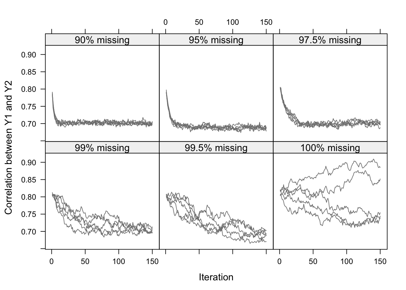

$Correlation between $Y_1$ and $Y_2$ in the imputed data per iteration in five independent runs of the MICE algorithm for six levels of missing data. The true value is 0.7. The figure illustrates that convergence can be slow for high percentages of missing data.$

Figure 4.3: Correlation between $Y_1$ and $Y_2$ in the imputed data per iteration in five independent runs of the MICE algorithm for six levels of missing data. The true value is 0.7. The figure illustrates that convergence can be slow for high percentages of missing data.

Figure 4.3 shows the development of $\rho(Y_1,Y_2)$ calculated on the completed data after every iteration of the MICE algorithm. At iteration 1, $\rho(Y_1,Y_2)$ is approximately 0.81, the value expected under independence of $Y_1$ and $Y_2$, conditional on $X$. The influence of the complete records with both $Y_1$ and $Y_2$ observed percolates into the imputations, so that the chains slowly move into the direction of the population value of 0.7. The speed of convergence heavily depends on the number of missing cases. For 90% or 95% missing data, the streams are essentially flat after about 15–20 iterations. As the percentage of missing data increases, more and more iterations are needed before the true correlation of 0.7 trickles through. In the extreme cases with 100% missing data, the correlation $\rho(Y_1,Y_2)$ cannot be estimated due to lack of information in the data. In this case, the different streams do not converge at all, and wander widely within the Cauchy–Schwarz bounds (0.6 to 1.0 here). But even here we could argue that the sampler has essentially converged. We could stop at iteration 200 and take the imputations from there. From a Bayesian perspective, this still would yield an essentially correct inference about $\rho(Y_1,Y_2)$, being that it could be anywhere within the Cauchy–Schwarz bounds. So even in this pathological case with 100% missing data, the results look sensible as long as we account for the wide variability.

The lesson we can learn from this simulation is that we should be careful about convergence in missing data problems with high correlations and high missing data rates. At the same time, observe that we really have to push the MICE algorithm to its limits to see the effect. Over 99% of real data will have lower correlations and lower missing data rates. Of course, it never hurts to do a couple of extra iterations, but my experience is that good results can often be obtained with a small number of iterations.

4.5.8 Performance

Each conditional density has to be specified separately, so FCS requires some modeling effort on the part of the user. Most software provides reasonable defaults for standard situations, so the actual effort required may be small. A number of simulation studies provide evidence that FCS generally yields estimates that are unbiased and that possess appropriate coverage (Brand 1999; Raghunathan et al. 2001; Brand et al. 2003; Tang et al. 2005; Van Buuren et al. 2006; Horton and Kleinman 2007; Yu, Burton, and Rivero-Arias 2007).