11.3 Time raster imputation
Longitudinal analysis has become virtually synonymous with mixed effects modeling. Following the influential work of Laird and Ware (1982) and Jennrich and Schluchter (1986), this approach characterizes individual growth trajectories by a small number of random parameters. The differences between individuals are expressed in terms of these parameters.
In some applications, it is natural to consider change scores. Change scores are however rather awkward within the context of mixed effects models. This section introduces time raster imputation, a new method to generate imputations on a regular time raster from irregularly spaced longitudinal data. The imputed data can then be used to calculate change scores or age-to-age correlations, or apply quantitative techniques designed for repeated measures.
11.3.1 Change score
Let \(Y_1\) and \(Y_2\) represent repeated measurements of the same object at times \(T_1\) and \(T_2\) where \(T_1<T_2\). The difference \(\Delta=Y_2-Y_1\) is the most direct measure of change over time. Willett (1989, 588) characterized the change score as an “intuitive, unbiased, and computationally-simple measure of individual growth.”
One would expect that modern books on longitudinal data would take the change score as their starting point. That is not the case. The change score is fully absent from most current books on longitudinal analysis. For example, there is no entry “change score” in the index of Verbeke and Molenberghs (2000), Diggle et al. (2002), Walls and Schafer (2006) or Fitzmaurice et al. (2009). Singer and Willett (2003, 10) do discuss the change score, but they quickly dismiss it on the basis that a study with only two time points cannot reveal the shape of a person’s growth trajectory.
The change score, once the centerpiece of longitudinal analysis, has disappeared from the methodological literature. I find this is somewhat unfortunate as the parameters in the mixed effects model are more difficult to interpret than the change score. Moreover, classic statistical techniques, like the paired \(t\)-test or split-plot ANOVA, are built on the change score. There is a gap between modern mixed effects models and classical linear techniques for change scores and repeated measures data.
Calculating a mean change score is only sensible if different persons are measured at the same time points. When the data are observed at irregular times, there is no simple way to calculate change scores. Calculating change scores from the person parameters of the mixed effects model is technically trivial, but such scores are difficult to interpret. The person parameters are fitted values that have been smoothed. Deriving a change score as the difference between the fitted curve of the person at \(T_1\) and \(T_2\) results in values that are closer to zero than those derived from data that have been observed.
This section describes a technique that inserts pseudo time points to the observed data of each person. The outcome data at these supplementary time points are multiply imputed. The idea is that the imputed data can be analyzed subsequently by techniques for change scores and repeated measures.
The imputation procedure is akin to the process needed to print a photo in a newspaper. The photo is coded as points on a predefined raster. At the microlevel there could be information loss, but the scenery is essentially unaffected. Hence the name time raster imputation. My hope is that this method will help bridge the gap between modern and classic approaches to longitudinal data.
11.3.2 Scientific question: Critical periods
The research was motivated by the question: At what ages do children become overweight? Knowing the answer to this question may provide handles for preventive interventions to counter obesity.
(Dietz 1994) suggested the existence of three critical periods for obesity at adult age: the prenatal period, the period of adiposity rebound (roughly around the age of 5-6 years), and adolescence. Obesity that begins at these periods is expected to increase the risk of persistent obesity and its complications. Overviews of studies on critical periods are given by Cameron and Demerath (2002) and Lloyd, Langley-Evans, and McMullen (2010).
In the sequel, we use the body mass index (BMI) as a measure of overweight. BMI will be analyzed in standard deviation scores (SDS) using the relevant Dutch references (Fredriks, Van Buuren, Burgmeijer, et al. 2000; Fredriks, Van Buuren, Wit, et al. 2000). Our criterion for being overweight in adulthood is defined as BMI SDS \(\geq\) 1.3.
As an example, imagine an 18-year-old person with a BMI SDS equal to +1.5 SD. How did this person end up at 1.5 SD? If we have the data, we can plot the measurements against age, and study the individual track. The BMI SDS trajectory may provide key insights into development of overweight and obesity.
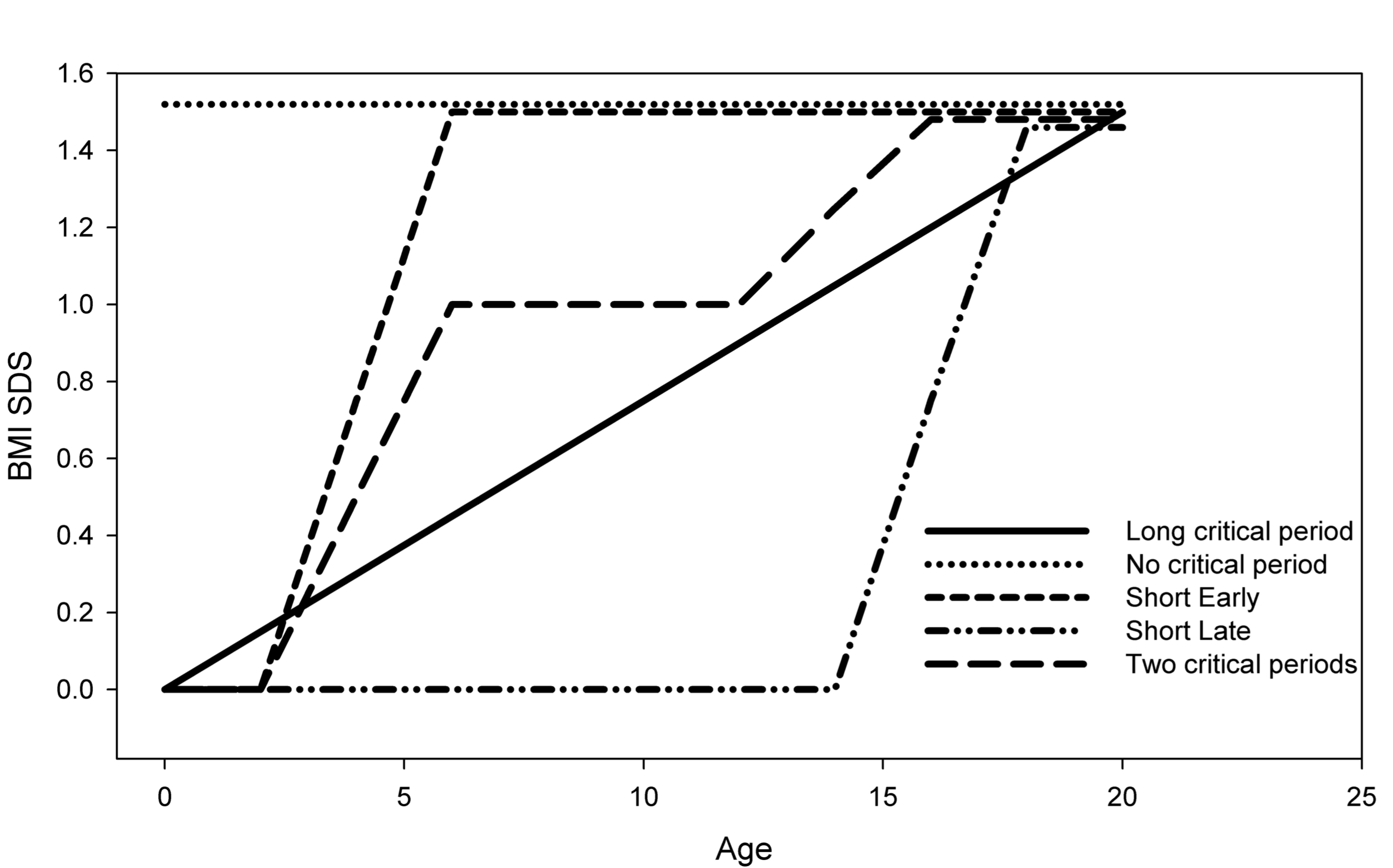
Figure 11.5: Five theoretical BMI SDS trajectories for a person age 18 years with a BMI SDS = 1.5 SD.
Figure 11.5 provides an overview of five theoretical BMI SDS trajectories that the person might have followed. These are:
Long critical period. A small but persistent centile crossing across the entire age range. In this case, everything (or nothing) is a critical period.
No critical period. The person is born with a BMI SDS of 1.5 SD and this remains unaltered throughout age.
Short early. There is a large increase between ages 2y and 5y. We would surely interpret the period 2y-5y is as a critical period for this person.
Short late. This is essentially the same as before, but shifted forward in time.
Two critical periods. Here the total increase of 1.5 SD is spread over two periods. The first occurs at 2y-5y with an increase of 1.0 SD. The second at 12y-15y with an increase of 0.5 SD.
In practice, mixing between these and other forms will occur.
The objective is to identify any periods during childhood that contribute to an increase in overweight at adult age. A period is “critical” if
change differs between those who are and are not later overweight; and
change is associated with the outcome after correction for the measure at the end of the period.
Both need to hold. In order to solve the problem of irregular age spacing, De Kroon et al. (2010) use the broken stick model, a piecewise linear growth curve fitted, as a means to describe individual growth curves at fixed times.
This section extends this methodology by generating imputations according to the broken stick model. The multiply imputed values are then used to estimate difference scores and regression models that throw light on the question of scientific interest.
11.3.3 Broken stick model\(^\spadesuit\)
In a sample of \(n\) persons \(i=1,\dots,n\), we assume that there are \(n_i\) measurement occasions for person \(i\). Let \(y_i\) represent the \(n_i\times 1\) vector containing the SDS values obtained for person \(i\). Let \(t_i\) represent the \(n_i\times 1\) vector with the ages at which the measurements were made.
The broken stick model requires the user to specify an ordered set of \(k\) break ages, collected in the vector \(\kappa=(\kappa_1,\dots,\kappa_k)\). The set should cover the entire range of the measured ages, so \(\kappa_1 \leq \min(t_i)\) and \(\kappa_k \geq \max(t_i)\) for all \(i\). It is convenient to set \(\kappa_1\) and \(\kappa_k\) to rounded values just below and above the minimum and maximum ages in the data, respectively. De Kroon et al. (2010) specified nine break ages: birth (0d), 8 days (8d), 4 months (4m), 1 year (1y), 2 years (2y), 6 years (6y), 10 years (10y), 18 years (18y) and 29 years (29y).
Without loss of information, the time points \(t_i\) of person \(i\) are represented by a \(B\)-spline of degree 1, with knots specified by \(\kappa\). More specifically, the vector \(t_i\) is recoded as the \(n_i\times k\) design matrix \(X_i=(x_{1i},\dots,x_{ki})\). We refer to Ruppert, Wand, and Carroll (2003, 59) for further details. For the set of break ages we calculate the \(B\)-splines matrix in R by the bs() function from the splines package as follows:
library(splines)
data <- tbc

### specify break ages
brk <- c(0, 8/365, 1/3, 1, 2, 6, 10, 18, 29)
k <- length(brk)

### calculate B-spline
X <- bs(data$age,
        knots = brk,
        B = c(brk[1], brk[k] + 0.0001),
        degree = 1)
X <- X[,-(k + 1)]
dimnames(X)[[2]] <- paste("x", 1:ncol(X), sep = "")
data <- cbind(data, X)
round(head(X, 3), 2)
x1 x2 x3 x4 x5 x6 x7 x8 x9
[1,] 1.00 0.00 0.00 0 0 0 0 0 0
[2,] 0.27 0.73 0.00 0 0 0 0 0 0
[3,] 0.00 0.83 0.17 0 0 0 0 0 0Matrix \(X\) has only two nonzero elements in each row. Each row sums to 1. If an observed age coincides with a break age, the corresponding entry is equal to 1, and all remaining elements are zero. In the data example, this occurs in the first record, at birth. A small constant of 0.0001 was added to the last break age. This was done to accommodate for a pseudo time point with an exact age of 29 years, which will be inserted later in Section 11.3.6.
The measurements \(y_i\) for person \(i\) are modeled by the linear mixed effects model
\[\begin{align} y_i & = X_i(\beta + \beta_i) + \epsilon_i \tag{11.2} \\ & = X_i\gamma_i + \epsilon_i \nonumber \end{align}\]where \(\gamma_i=\beta + \beta_i\). The \(k\times 1\) column vector \(\beta\) contains \(k\) fixed-effect coefficients common to all persons. The vector \(\beta_i\) contains \(k\) subject-specific random effect coefficients for person \(i\). The vector \(\epsilon_i\) contains \(n_i\) subject-specific residuals.
We make the usual assumption that \(\gamma_i\sim N(\beta,\Omega)\), i.e., the random coefficients of the subjects have a multivariate normal distribution with global mean \(\beta\) and an unstructured covariance \(\Omega\). We also assume that the residuals are independently and normally distributed as \(\epsilon_i \sim N(0,\sigma^2 I(n_i))\) where \(\sigma^2\) is a common variance parameter. The covariances between \(\beta_i\) and \(e_i\) are assumed to be zero.
Since the rows of the \(B\)-spline basis all sum to 1, the intercept is implicit. In fact, one could interpret the model as a special form of the random intercept model, where the intercept is represented by a \(B\)-spline rather than by the usual column of ones.
The model prescribes that growth follows a straight line between the break ages. In this application, we are not so much interested in what happens within the age interval of each period. Rogosa and Willett (1985) contrasted the analysis of individual differences based on change scores with the analysis of individual differences based on multilevel parameters. They concluded that in general the analysis of change scores is inferior to the parameter approach. The exception is when growth is assumed to follow a straight line within the interval of interest. In that case, the change score approach and the mixed effects model are interchangeable (Rogosa and Willett 1985, 225). The straight line assumption is often reasonable in epidemiological studies if the time interval is short (Hui and Berger 1983). For extra detail, we could add an extra break age within the interval.
The function lmer() from the lme4 package fits the model. Change scores can be calculated from the fixed and random effects as follows:
library(lme4)
fit <- lmer(wgt.z ~ 0 + x1 + x2 + x3 + x4 + x5 +
              x6 + x7 + x8 + x9 + (0 + x1 + x2 +
              x3 + x4 + x5 + x6 + x7 + x8 + x9 | id),
            data = data)

### calculate size and increment per person
tsiz <- t(ranef(fit)$id) + fixef(fit)
tinc <- diff(tsiz)

round(head(t(tsiz)), 2)
The \(\hat\gamma_i\) estimates are found in the variable tsiz. Let \(\hat\delta_{ik}=\hat\gamma_{i,j+1}-\hat\gamma_{i,j}\) with \(j=1,\dots,k-1\) denote the successive differences (or increments) of the elements in \(\hat\gamma_i\). These are found in the variable tinc. We may interpret \(\hat\delta_i\) as the expected change scores for person \(i\).
The first criterion for a critical period is that change differs between those who are and are not later overweight. A simple analysis for this criterion is the Student’s \(t\)-test applied to \(\hat\delta_{ik}\) for every period \(k\). The correlations between \(\hat\delta_{ik}\) at successive \(k\) were generally higher than 0.5, so we analyzed unconditional change scores (Jones and Spiegelhalter 2009). The second criterion for a critical period involves fitting two regression models, both of which have final BMI SDS at adulthood, denoted by \(\gamma_i^\mathrm{adult}\), as their outcome. The two models are:
\[\begin{align} \gamma_i^\mathrm{adult} & = \hat\gamma_{i,j+1}\zeta_{j+1} + \epsilon_i \\ \gamma_i^\mathrm{adult} & = \hat\gamma_{i,j+1}\eta_{j+1} + \hat\gamma_j\eta_j + \varepsilon_i \end{align}\]which are fitted for \(j=1,\dots,k-2\). The parameter of scientific interest is the added value of including \(\eta_j\).
11.3.4 Terneuzen Birth Cohort
The Terneuzen Birth Cohort consists of all (\(n\) = 2604) newborns in Terneuzen, the Netherlands, between 1977 and 1986. The most recent measurements were made in the year 2005, so the data spans an age range of 0-29 years. Height and weight were measured throughout this age range. More details on the measurement procedures and the data can be found in De Kroon et al. (2008; De Kroon et al. 2010).
Suppose the model is fitted to weight SDS. The parameters \(\gamma_i\) can be interpreted as attained weight SDS relative to the reference population. This allows us to represent the observed trajectory of each child in a condensed way by \(k\) numbers. The values in \(\hat\gamma_i\) are the set of most likely weight SDS values at each break age, given all true measurements we have of child \(i\). This implies that if the child has very few measurements, the estimates will be close to the global mean. When taken together, the values \(\hat\gamma_i\) form the broken stick.
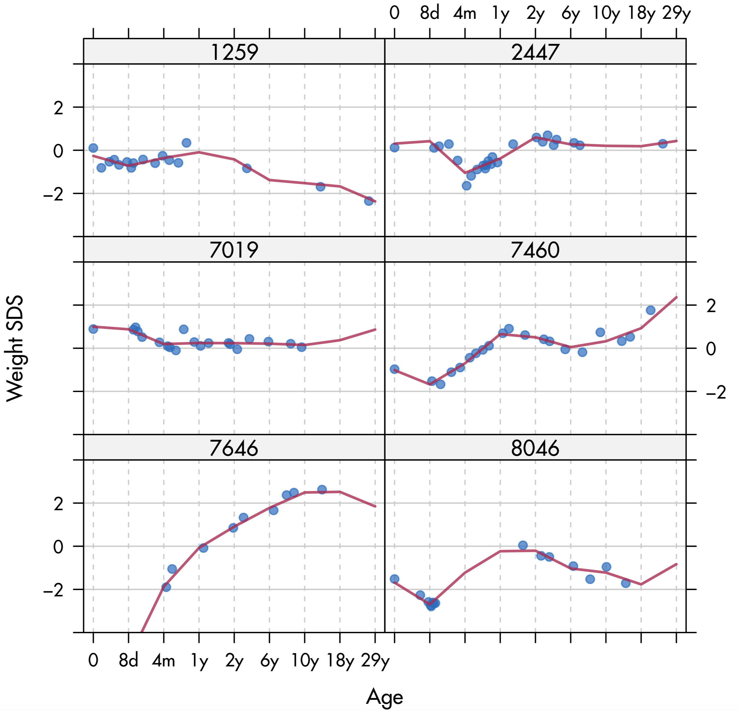
Figure 11.6: Broken stick trajectories for weight SDS from six selected individuals from the Terneuzen cohort.
Figure 11.6 displays weight SDS against age for six selected individuals. Child 1259 has a fairly common pattern. This child starts off near the average, but then steadily declines, apart from a blip around 10months. Child 2447 is fairly constant, but had a major valley near the age of 4months, perhaps because of a temporary illness. Child 7019 is also typical. The pattern hovers around the mean. Observe that no data beyond 10 years are available for this child. Child 7460 experienced a substantial change in the height/weight proportions during the first year. Child 7646 was born prematurely with a gestational age of 32 weeks. This individual has an unusually large increase in weight between birth and puberty. Child 8046 is aberrant with an unusually large number of weight measurements around the age of 8 days, but was subsequently not measured for about 1.5 years.
Figure 11.6 also displays the individual broken stick estimates for each outcome as a line. Observe that the model follows the individual data points very well. De Kroon et al. (2010) analyzed these estimates by the methods described at the end of Section 11.3.2, and found that the periods 2y-6y and 10y-18y were most relevant for developing later overweight.
11.3.5 Shrinkage and the change score\(^\spadesuit\)
Thus far we have looked at the problem from a prediction perspective. This is a useful first step, but it does not address all aspects. The \(\hat\beta_i\) estimate in the mixed effects model combines the person-specific ordinary least squares (OLS) estimate of \(\beta_i\) with the grand mean \(\hat\beta\). The amount of shrinkage toward the grand mean depends on three factors: the number of data points \(n_i\), the residual variance estimate \(\hat\sigma^2\) around the fitted broken stick, and the variance estimate \(\hat\omega_j^2\) for the \(j^\mathrm{th}\) random effect. If \(n_i=\sigma^2/\hat\omega_j^2\) then \(\hat\beta_i\) is halfway between \(\hat\beta\) and the OLS estimate of \(\beta_i\). If \(n_i < \hat\sigma^2/\omega_j^2\) then \(\hat\beta_i\) is closer to the global mean, while \(n_i > \hat\sigma^2/\hat\omega_j^2\) implies that \(\hat\beta_i\) is closer to the OLS-estimate. We refer to Gelman and Hill (2007, 394) for more details.
Shrinkage will stabilize the estimates of persons with few data points. Shrinkage also implies that the same \(\hat\gamma_i = \hat\beta+\hat\beta_i\) can correspond to quite different data trajectories. Suppose profile A is an essentially flat and densely measured trajectory just above the mean. Profile B, on the other hand, is a sparse and highly variable trajectory far above the mean. Due to differential shrinkage, profiles A and B can have the same \(\hat\gamma_i\) estimates. As a consequence, shrinkage will affect the change scores \(\hat\delta_i\). For both profiles A and B the estimated change scores \(\hat\delta_i\) are approximately zero at every period. For profile A this is reasonable since the profile itself is flat. In profile B we would expect to see substantial variation in \(\hat\delta_i\) if the data had been truly measured. Yet, shrinkage has dampened \(\hat\gamma_i\), and thus made \(\hat\delta_i\) closer to zero than if calculated from observed data.
It is not quite known whether this effect is a problem in this application. It is likely that dampening of \(\hat\delta_i\) will bias the result in the conservative direction, and hence primarily affects statistical power. The next section explores an alternative based on multiple imputation. The idea is to insert the break ages into the data, and impute the corresponding outcome data.
11.3.6 Imputation
The measured outcomes are denoted by \(Y_\mathrm{obs}\), e.g., weight SDS. For the moment, we assume that the \(Y_\mathrm{obs}\) are coded in long format and complete, though neither is an essential requirement. For each person \(i\) we append \(k\) records, each of which corresponds to a break age. In R we first set up a time warping model that connect real age to warped age, and then integrate the new ages into the data.
warp.setup <- data.frame(age = brk,
                         age2 = seq(0, 29, length.out=k))
warp.model <- lm(
  age2 ~ bs(age, knots = brk[c(-1, -k)], degree = 1) - 1,
  data = warp.setup, x = TRUE, y = TRUE)
warped.knots <- warp.model$y
maxage <- max(warped.knots)
age2  <- predict(warp.model, newdata = data)
data  <- cbind(data, age2 = age2)
rm(age2)
id <- unique(data$id)
data2 <- appendbreak(data, brk, id = id,
                     warp.model = warp.model, typ = "sup")
table(data2$typ)
  obs   sup  pred
32845 15705     0
The function appendbreak() is a custom function of about 20 lines in mice specific to the Terneuzen Birth Cohort data. It copies the first available record of the \(i^\mathrm{th}\) person \(k\) times, updates administrative and age variables, sets the outcome variables to NA, appends the result to the original data and sorts the result with respect to id and age. The real data are thus mingled with the supplementary records with missing outcomes. The first few records of data2 look like this:
head(data2) id occ nocc first typ age sex hgt.z wgt.z bmi.z ao x1
4 4 0 19 TRUE obs 0.000 1 0.33 0.195 0.666 0 1.00
42 4 NA 19 FALSE sup 0.000 1 NA NA NA 0 1.00
5 4 1 19 FALSE obs 0.016 1 NA -0.666 NA 0 0.27
4.1 4 NA 19 FALSE sup 0.022 1 NA NA NA 0 0.00
6 4 2 19 FALSE obs 0.076 1 0.71 0.020 -0.381 0 0.00
7 4 3 19 FALSE obs 0.104 1 0.18 0.073 0.075 0 0.00
x2 x3 x4 x5 x6 x7 x8 x9 age2
4 0.00 0.00 0 0 0 0 0 0 0.0
42 0.00 0.00 0 0 0 0 0 0 0.0
5 0.73 0.00 0 0 0 0 0 0 2.6
4.1 1.00 0.00 0 0 0 0 0 0 3.6
6 0.83 0.17 0 0 0 0 0 0 4.3
7 0.74 0.26 0 0 0 0 0 0 4.6Multiple imputation must take into account that the data are clustered within persons. The setup for mice() requires some care, so we discuss each step in detail.
Y <- c("hgt.z", "wgt.z", "bmi.z")
meth <- make.method(data2)
meth[1:length(meth)] <- ""
meth[Y] <- "2l.pan"
These statements specify that only hgt.z, wgt.z and bmi.z need to be imputed. For these three outcomes we request the elementary imputation function mice.impute.2l.pan(), which is designed to impute data with two levels. See Section 7.6 for more detail.
pred <- make.predictorMatrix(data2)
pred[1:nrow(pred), 1:ncol(pred)] <- 0
pred[Y, "id"] <- (-2)
pred[Y, "sex"] <- 1
pred[Y, paste("x", 2:9, sep = "")] <- 1
pred[Y[1], Y[2]] <- 1
pred[Y[2], Y[1]] <- 1
pred[Y[3], Y[1:2]] <- 1
The setup of the predictor matrix needs some care. We first empty all entries from the variable pred. The statement pred[Y, id] <- (-2) defines variable id as the class variable. The statement pred[Y, sex] <- 1 specifies sex as a fixed effect, as usual, while pred[Y, paste(x, 1:9, sep = )] <- 2 sets the \(B\)-spline basis as a random effect, as in Equation (11.2). The remaining three statement specify the \(Y_2\) is a random effects predictor of \(Y_1\) (and vice versa), and both \(Y_1\) and \(Y_2\) are random effects predictors of \(Y_3\). Note that \(Y_3\) (BMI SDS) is not a predictor of \(Y_1\) or \(Y_2\) in order to prevent the type of convergence problems explained in Section 6.5.2. Note also that age is not included in order to evade duplication with its \(B\)-spline coding. In summary, there are 12 random effects (9 for age and 3 for the outcomes), one class variable, and one fixed effect.
The actual imputations are produced by
imp.1745 <- mice(data2, meth = meth, pred = pred, m = 10,
                 maxit = 10, seed = 52711, print = FALSE)
There are over 48000 records. This call takes about 30 minutes to complete, which is much longer than the other applications discussed in this book. In the year 2012 the same problem still took over 10 hours, so there is certainly progress.
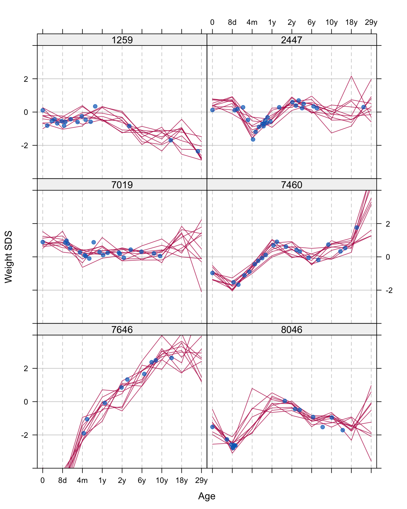
Figure 11.7: Ten multiply imputed trajectories of weight SDS for the same persons as in Figure 11.6 (in red). Also shown are the data points (in blue).
Figure 11.7 displays ten multiply imputed trajectories for the six persons displayed in Figure 11.6. The general impression is that the imputed trajectory follows the data quite well. At ages where the are many data points (e.g., in period 0d-1y in person 1259 or in period 8d-1y in person 7460) the curves are quite close, indicating a relatively large certainty. On the other hand, at locations where data are sparse (e.g., the period 10y-29y in person 7019, or the period 8d-2y in person 8046) the curves diverge, indicating a large amount of uncertainty about the imputation. This effect is especially strong at the edges of the age range. Incidentally, we noted that the end effects are less pronounced for larger sample sizes.
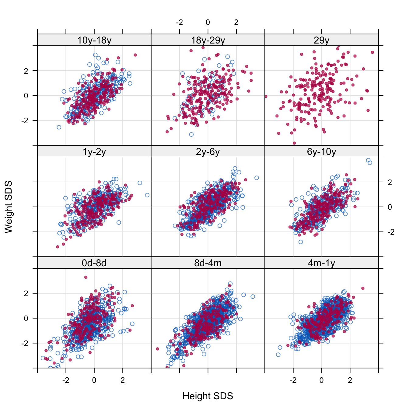
Figure 11.8: The relation between height SDS and weight SDS in the observed (blue) and imputed (red) longitudinal trajectories. The imputed data occur exactly at the break ages. The observed data come from the period immediately after the break age. No data beyond 29 years were observed, so the upper-right panel contains no observed data.
It is also interesting to study whether imputation preserves the relation between height, weight and BMI. Figure 11.8 is a scattergram of height SDS and weight SDS split according to age that superposes the imputations on the observed data in the period after the break point. In general the relation in the observed data is preserved in the imputed data. Note that the imputations become more variable for regions with fewer data. This is especially visible at the panel in the upper-right corner at age 29y, where there were no data at all. Similar plots can be made in combination with BMI SDS. In general, the data in these plots all behave as one would expect.
11.3.7 Complete-data model
Table 11.2 provides a comparison of the mean changes observed under the broken stick model and under time raster imputation. The estimates are very similar, so the mean change estimated under both methods is similar. The \(p\)-values in the broken stick method are generally more optimistic relative to multiple imputation, which is due to the fact that the broken stick model ignores the uncertainty about the estimates.
| Broken stick | Time raster imputation | |||||
| Period | NAO | AO | \(p\)-value | NAO | AO | \(p\)-value |
| 0d-8d | -0.88 | -0.80 | 0.214 | -0.93 | -0.82 | 0.335 |
| 8d-4m | -0.32 | -0.34 | 0.811 | -0.07 | -0.11 | 0.745 |
| 4m-1y | 0.42 | 0.62 | 0.006 | 0.35 | 0.58 | 0.074 |
| 1y-2y | 0.22 | 0.28 | 0.242 | 0.24 | 0.26 | 0.884 |
| 2y-6y | -0.36 | -0.10 | <0.001 | -0.35 | -0.06 | 0.026 |
| 6y-10y | 0.05 | 0.34 | <0.001 | -0.01 | 0.31 | 0.029 |
| 10y-18y | 0.09 | 0.52 | <0.001 | 0.17 | 0.68 | 0.009 |
There is also an effect on the correlations. In general, the age-to-age correlations of the broken stick method are higher than the raster imputations.
| Age | 0d | 8d | 4m | 1y | 2y | 6y | 10y | 18y |
|---|---|---|---|---|---|---|---|---|
| 0d | - | 0.64 | 0.20 | 0.21 | 0.18 | 0.17 | 0.16 | 0.11 |
| 8d | 0.75 | - | 0.30 | 0.17 | 0.20 | 0.20 | 0.15 | 0.13 |
| 4m | 0.28 | 0.44 | - | 0.39 | 0.30 | 0.29 | 0.20 | 0.16 |
| 1y | 0.28 | 0.23 | 0.65 | - | 0.55 | 0.40 | 0.31 | 0.23 |
| 2y | 0.31 | 0.33 | 0.46 | 0.76 | - | 0.56 | 0.36 | 0.23 |
| 6y | 0.31 | 0.36 | 0.46 | 0.59 | 0.79 | - | 0.62 | 0.42 |
| 10y | 0.26 | 0.26 | 0.35 | 0.47 | 0.55 | 0.89 | - | 0.53 |
| 18y | 0.23 | 0.26 | 0.29 | 0.37 | 0.40 | 0.72 | 0.89 | - |
Table 11.3 provides the age-to-age correlation matrix of BMI SDS estimated from 1745 cases from the Terneuzen Birth Cohort. Apart from the peculiar values for the age of 8 days, the correlations decrease as the period between time points increases. The values for the broken stick method are higher because these do not incorporate the uncertainty of the estimates.