2.2 Concepts in incomplete data

2.2.1 Incomplete-data perspective

Many statistical techniques address some kind of incomplete-data problem. Suppose that we are interested in knowing the mean income \(Q\) in a given population. If we take a sample from the population, then the units not in the sample will have missing values because they will not be measured. It is not possible to calculate the population mean right away since the mean is undefined if one or more values are missing. The incomplete-data perspective is a conceptual framework for analyzing data as a missing data problem.

Estimating a mean from a population is a well known problem that can also be solved without a reference to missing data. It is nevertheless sometimes useful to think what we would have done had the data been complete, and what we could do to arrive at complete data. The incomplete-data perspective is general, and covers the sampling problem, the counterfactual model of causal inference, statistical modeling of the missing data, and statistical computation techniques. The books by Gelman et al. (2004 ch. 7) and Gelman and Meng (2004) provide in-depth discussions of the generality and richness of the incomplete data perspective. Little (2013) lists ten powerful ideas for the statistical scientist. His final advice reads as:

My last simple idea is overarching: statistics is basically a missing data problem! Draw a picture of what’s missing and find a good model to fill it in, along with a suitable (hopefully well calibrated) method to reflect uncertainty.

2.2.2 Causes of missing data

There is a broad distinction between two types of missing data: intentional and unintentional missing data. Intentional missing data are planned by the data collector. For example, the data of a unit can be missing because the unit was excluded from the sample. Another form of intentional missing data is the use of different versions of the same instrument for different subgroups, an approach known as matrix sampling. See Gonzalez and Eltinge (2007) or Graham (2012 Section 4) for an overview. Also, missing data that occur because of the routing in a questionnaire are intentional, as well as data (e.g., survival times) that are censored data at some time because the event (e.g., death) has not yet taken place. A related term in a multilevel context is systematically missing data. This term refers to variables that are missing for all individuals in a cluster because the variable was not measured in that cluster.(Resche-Rigon and White 2018)

Though often foreseen, unintentional missing data are unplanned and not under the control of the data collector. Examples are: the respondent skipped an item, there was an error in the data transmission causing data to be missing, some of the objects dropped out before the study could be completed resulting in partially complete data, and the respondent was sampled but refused to cooperate. A related term in a multilevel context is sporadically missing data. This terms is used for variables with missing values for some but not all individuals in a cluster.

Another important distinction is item nonresponse versus unit nonresponse. Item nonresponse refers to the situation in which the respondent skipped one or more items in the survey. Unit nonresponse occurs if the respondent refused to participate, so all outcome data are missing for this respondent. Historically, the methods for item and unit nonresponse have been rather different, with unit nonresponse primarily addressed by weighting methods, and item nonresponse primarily addressed by edit and imputation techniques.

Table 2.1: Examples of reasons for missingness for combinations of intentional/unintentional missing data with item/unit nonresponse.

	Intentional	Unintentional
Unit nonresponse	Sampling	Refusal
		Self-selection
Item nonresponse	Matrix sampling	Skip question
	Branching	Coding error

Table 2.1 cross-classifies both distinctions, and provides some typical examples in each of the four cells. The distinction between intentional/unintentional missing data is the more important one. The item/unit nonresponse distinction says how much information is missing, while the distinction between intentional and unintentional missing data says why some information is missing. Knowing the reasons why data are incomplete is a first step toward the solution.

2.2.3 Notation

The notation used in this book will be close to that of Rubin (1987b) and Schafer (1997), but there are some exceptions. The symbol \(m\) is used to indicate the number of multiple imputations. Compared to Rubin (1987b) the subscript \(m\) is dropped from most of the symbols. In Rubin (1987b), \(Y\) and \(R\) represent the data of the population, whereas in this book \(Y\) refers to data of the sample, similar to Schafer (1997). Rubin (1987b) uses \(X\) to represent the completely observed covariates in the population. Here we assume that the covariates are possibly part of \(Y\), so there is not always a symbolic distinction between complete covariates and incomplete data. The symbol \(X\) is used to indicate the set of predictors in various types of models.

Let \(Y\) denote the \(n \times p\) matrix containing the data values on \(p\) variables for all \(n\) units in the sample. We define the response indicator \(R\) as an \(n \times p\) 0–1 matrix. The elements of \(Y\) and \(R\) are denoted by \(y_{ij}\) and \(r_{ij}\), respectively, where \(i=1,\dots,n\) and \(j=1,\dots,p\). If \(y_{ij}\) is observed, then \(r_{ij} = 1\), and if \(y_{ij}\) is missing, then \(r_{ij} = 0\).

This book is restricted to the case where \(R\) is completely known, i.e., we know where the missing data are. This covers many applications of practical interest, but not all. For example, some questionnaires present a list of diseases and ask the respondent to place a “tick” at each disease that applies. If there is a “yes” we know that the field is not missing. However, if the field is not ticked, it could be because the person didn’t have the disease (a genuine “no”) or because the respondent skipped the question (a missing value). There is no way to tell the difference from the data, so these are unknown unknowns. In order to make progress in cases like these, we need additional assumptions about the response behavior.

The observed data are collectively denoted by \(Y_\mathrm{obs}\). The missing data are collectively denoted as \(Y_\mathrm{mis}\), and contain all elements \(y_{ij}\) where \(r_{ij}=0\). When taken together \(Y=(Y_\mathrm{obs},Y_\mathrm{mis})\) contain the hypothetically complete data. The part \(Y_\mathrm{mis}\) has real values, but the values themselves are masked from us, where \(R\) indicates which values are masked. In their book, Little and Rubin (2002, 8) make the following key assumption:

Missingness indicators hide the true values that are meaningful for analysis.

While this statement may seem obvious and uncomplicated, there are practical situations where it may not hold. In a trial where we are interested in both survival and quality of life, we may have missing values in either outcome. If we know that a person is alive, then an unknown quality of life outcome is simply missing because the quality of life score is defined for that person, but for some reason we haven’t been able to see it. But if the person has died, quality of life becomes undefined, and that’s the reason why we don’t see it. It wouldn’t make much sense to try to impute something that is undefined. A more sensible option is to stratify the analysis according to whether the concept is defined or not. The situation becomes more complex if we do not know the person’s survival status. See Rubin (2000) for an analysis. In order to evade such complexities, we assume that \(Y\) contains values that are all defined, and that \(R\) indicates what we actually see.

If \(Y=Y_\mathrm{obs}\) (i.e., if the sample data are completely observed) and if we know the mechanism of how the sample was created, then it is possible to make a valid estimate of the population quantities of interest. For a simple random sample, we could just take the sample mean \(\hat Q\) as an unbiased estimate of the population mean \(Q\). We will assume throughout this book that we know how to do the correct statistical analysis on the complete data \(Y\). If we cannot do this, then there is little hope that we can solve the more complex problem of analyzing \(Y_\mathrm{obs}\). This book addresses the problem of what to do if \(Y\) is observed incompletely. Incompleteness can incorporate intentional missing data, but also unintentional forms like refusals, self-selection, skipped questions, missed visits and so on.

Note that every unit in the sample has a row in \(Y\). If no data have been obtained for a unit \(i\) (presumably because of unit nonresponse), the \(i^\mathrm{th}\) record will contain only the sample number and perhaps administrative data from the sampling frame. The remainder of the record will be missing.

A variable without any observed values is called a latent variable. Latent variables are often used to define concepts that are difficult to measure. Latent variables are theoretical constructs and not part of the manifest data, so they are typically not imputed. Mislevy (1991) showed how latent variable can be imputed, and provided several illustrative applications.

2.2.4 MCAR, MAR and MNAR again

Section 1.2 introduced MCAR, MAR and MNAR. This section provides more precise definitions.

The matrix \(R\) stores the locations of the missing data in \(Y\). The distribution of \(R\) may depend on \(Y=(Y_\mathrm{obs}, Y_\mathrm{mis})\), either by design or by happenstance, and this relation is described by the missing data model. Let \(\psi\) contain the parameters of the missing data model, then the general expression of the missing data model is \(\Pr(R|Y_\mathrm{obs},Y_\mathrm{mis},\psi)\).

The data are said to be MCAR if

\[\begin{equation} \Pr(R=0|{\mbox{$Y_\mathrm{obs}$}},{\mbox{$Y_\mathrm{mis}$}},\psi) = \Pr(R=0|\psi) \tag{2.1} \end{equation}\]

so the probability of being missing depends only on some parameters \(\psi\), the overall probability of being missing. The data are said to be MAR if

\[\begin{equation} \Pr(R=0|{\mbox{$Y_\mathrm{obs}$}},{\mbox{$Y_\mathrm{mis}$}},\psi) = \Pr(R=0|{\mbox{$Y_\mathrm{obs}$}},\psi) \tag{2.2} \end{equation}\]

so the missingness probability may depend on observed information, including any design factors. Finally, the data are MNAR if

\[\begin{equation} \Pr(R=0|{\mbox{$Y_\mathrm{obs}$}},{\mbox{$Y_\mathrm{mis}$}},\psi) \tag{2.3} \end{equation}\]

does not simplify, so here the probability to be missing also depends on unobserved information, including \(Y_\mathrm{mis}\) itself.

As explained in Chapter 1, simple techniques usually only work under MCAR, but this assumption is very restrictive and often unrealistic. Multiple imputation can handle both MAR and MNAR.

Several tests have been proposed to test MCAR versus MAR. These tests are not widely used, and their practical value is unclear. See Enders (2010, 17–21) for an evaluation of two procedures. It is not possible to test MAR versus MNAR since the information that is needed for such a test is missing.

Numerical illustration. We simulate three archetypes of MCAR, MAR and MNAR. The data \(Y=(Y_1,Y_2)\) are drawn from a standard bivariate normal distribution with a correlation between \(Y_1\) and \(Y_2\) equal to 0.5. Missing data are created in \(Y_2\) using the missing data model

\[\begin{equation} \Pr(R_2=0)=\psi_0+\frac{e^{Y_1}}{1+e^{Y_1}}\psi_1+\frac{e^{Y_2}}{1+e^{Y_2}}\psi_2 \tag{2.4} \end{equation}\]

with different parameters settings for \(\psi=(\psi_0,\psi_1,\psi_2)\). For MCAR we set \(\psi_\mathrm{MCAR}=(0.5,0,0)\), for MAR we set \(\psi_\mathrm{MAR}=(0,1,0)\) and for MNAR we set \(\psi_\mathrm{MNAR}=(0,0,1)\). Thus, we obtain the following models:

\[\begin{align} \mathrm{MCAR}&:&\mathrm{}\Pr(R_2=0) = 0.5 \tag{2.5}\\ \mathrm{MAR}&:&\mathrm{logit}(\Pr(R_2=0)) = Y_1 \tag{2.6}\\ \mathrm{MNAR}&:&\mathrm{logit}(\Pr(R_2=0)) = Y_2 \tag{2.7}\\ \end{align}\]

where \(\mathrm{logit}(p)=\log(p/(1-p))\) for any \(0 < p < 1\) is the logit function. In practice, it is more convenient to work with the inverse logit (or logistic) function inverse \(\mathrm{logit}^{-1}(x) = \exp(x)/(1+\exp(x))\), which transforms a continuous \(x\) to the interval \(\langle 0,1\rangle\). In R, it is straightforward to draw random values under these models as

logistic <- function(x) exp(x) / (1 + exp(x))
set.seed(80122)
n <- 300
y <- MASS::mvrnorm(n = n, mu = c(0, 0),
                   Sigma = matrix(c(1, 0.5, 0.5, 1), nrow = 2))
r2.mcar <- 1 - rbinom(n, 1, 0.5)
r2.mar  <- 1 - rbinom(n, 1, logistic(y[, 1]))
r2.mnar <- 1 - rbinom(n, 1, logistic(y[, 2]))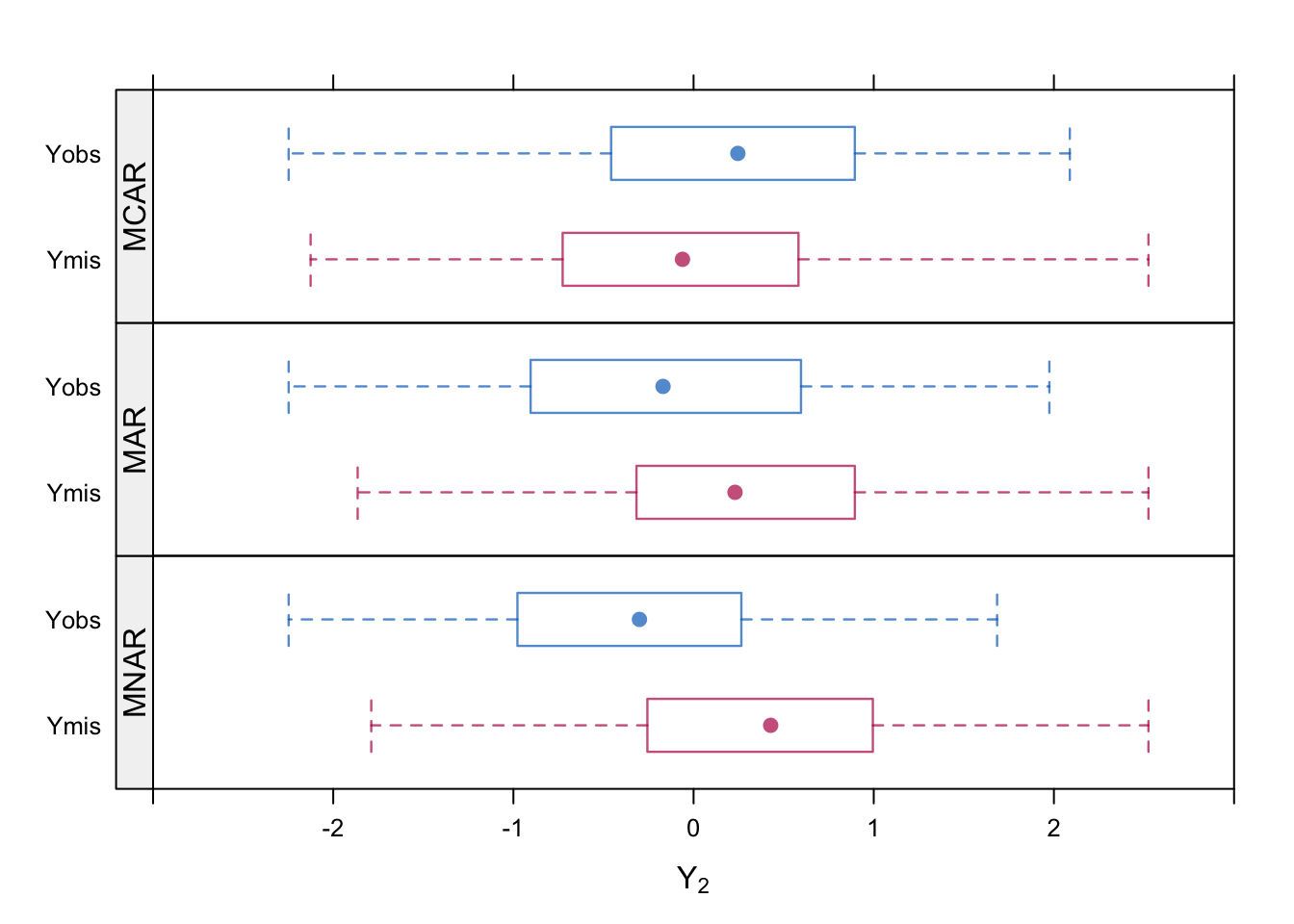

Figure 2.2: Distribution of \(Y_\mathrm{obs}\) and \(Y_\mathrm{mis}\) under three missing data models.

Figure 2.2 displays the distribution of \(Y_\mathrm{obs}\) and \(Y_\mathrm{mis}\) under the three missing data models. As expected, these are similar under MCAR, but become progressively more distinct as we move to the MNAR model.

2.2.5 Ignorable and nonignorable\(^\spadesuit\)

The example in the preceding section specified parameters \(\psi\) for three missing data models. The \(\psi\)-parameters have no intrinsic scientific value and are generally unknown. It would simplify the analysis if we could just ignore these parameters. The practical importance of the distinction between MCAR, MAR and MNAR is that it clarifies the conditions under which we can accurately estimate the scientifically interesting parameters without the need to know \(\psi\).

The actually observed data consist of \(Y_\mathrm{obs}\) and \(R\). The joint density function \(f(Y_\mathrm{obs}, R|\theta,\psi)\) of \(Y_\mathrm{obs}\) and \(R\) together depends on parameters \(\theta\) for the full data \(Y\) that are of scientific interest, and parameters \(\psi\) for the response indicator \(R\) that are seldom of interest. The joint density is proportional to the likelihood of \(\theta\) and \(\psi\), i.e.,

\[\begin{equation} l(\theta,\psi|{\mbox{$Y_\mathrm{obs}$}},R) \propto f({\mbox{$Y_\mathrm{obs}$}}, R|\theta,\psi) \tag{2.8} \end{equation}\]

The question is: When can we determine \(\theta\) without knowing \(\psi\), or equivalently, the mechanism that created the missing data? The answer is given in Little and Rubin (2002, 119):

The missing data mechanism is ignorable for likelihood inference if:

1. MAR: the missing data are missing at random; and

2. Distinctness: the parameters \(\theta\) and \(\psi\) are distinct, in the sense that the joint parameter space of \((\psi,\theta)\) is the product of the parameter space of \(\theta\) and the parameter space of \(\psi\).

For valid Bayesian inference, the latter condition is slightly stricter: \(\theta\) and \(\psi\) should be a priori independent: \(p(\theta,\psi) = p(\theta)p(\psi)\) (Little and Rubin 2002, 120). The MAR requirement is generally considered to be the more important condition. Schafer (1997, 11) says that in many situations the condition on the parameters is “intuitively reasonable, as knowing \(\theta\) will provide little information about \(\psi\) and vice-versa.” We should perhaps be careful in situations where the scientific interest focuses on the missing data process itself. For all practical purposes, the missing data model is said to be “ignorable” if MAR holds.

Note that the label “ignorable” does not mean that we can be entirely careless about the missing data. For inferences to be valid, we need to condition on those factors that influence the missing data rate. For example, in the MAR example of Section 2.2.4 the missingness in \(Y_2\) depends on \(Y_1\). A valid estimate of the mean of \(Y_2\) cannot be made without \(Y_1\), so we should include \(Y_1\) somehow into the calculations for the mean of \(Y_2\).

2.2.6 Implications of ignorability

The concept of ignorability plays an important role in the construction of imputation models. In imputation, we want to draw synthetic observations from the posterior distribution of the missing data, given the observed data and given the process that generated the missing data. The distribution is denoted as \(P(Y_\mathrm{mis}|Y_\mathrm{obs},R)\). If the nonresponse is ignorable, then this distribution does not depend on \(R\) (Rubin 1987b Result 2.3), i.e.,

\[\begin{equation} P({\mbox{$Y_\mathrm{mis}$}}|{\mbox{$Y_\mathrm{obs}$}}, R) = P({\mbox{$Y_\mathrm{mis}$}}|{\mbox{$Y_\mathrm{obs}$}}) \tag{2.9} \end{equation}\]

The implication is that

\[\begin{equation} P(Y|{\mbox{$Y_\mathrm{obs}$}}, R=1) = P(Y|{\mbox{$Y_\mathrm{obs}$}}, R=0) \tag{2.10} \end{equation}\]

so the distribution of the data \(Y\) is the same in the response and nonresponse groups. Thus, if the missing data model is ignorable we can model the posterior distribution \(P(Y|Y_{\mathrm{obs}}, R=1)\) from the observed data, and use this model to create imputations for the missing data. Vice versa, techniques that (implicitly) assume equivalent distributions assume ignorability and thus MAR. On the other hand, if the nonresponse is nonignorable, we find

\[\begin{equation} P(Y|{\mbox{$Y_\mathrm{obs}$}}, R=1) \not= P(Y|{\mbox{$Y_\mathrm{obs}$}}, R=0) \tag{2.11} \end{equation}\]

so then we should incorporate \(R\) into the model to create imputations.

The assumption of ignorability is often sensible in practice, and generally provides a natural starting point. If, on the other hand, the assumption is not reasonable (e.g., when data are censored), we may specify \(P(Y|Y_\mathrm{obs}, R=0)\) different from \(P(Y|Y_\mathrm{obs}, R=1)\). The specification of \(P(Y|Y_\mathrm{obs}, R=0)\) needs assumptions external to the data since, by definition, the information needed to estimate any regression weights for \(R\) is missing.

Example. Suppose that a growth study measures body weight in kg (\(Y_2\)) and gender (\(Y_1\): 1 = boy, 0 = girl) of 15-year-old children, and that some of the body weights are missing. We can model the weight distribution for boys and girls separately for those with observed weights, i.e., \(P(Y_2 | Y_1=1, R_2=1)\) and \(P(Y_2 | Y_1=0, R_2=1)\). If we assume that the response mechanism is ignorable, then imputations for a boy’s weight can be drawn from \(P(Y_2 | Y_1=1, R_2=1)\) since it will equal \(P(Y_2 | Y_1=1, R_2=0)\). The same can be done for the girls. This procedure leads to correct inferences on the combined sample of boys and girls, even if boys have substantially more missing values, or if the body weights of the boys and girls are very different.

The procedure outlined above is not appropriate if, within the boys or the girls, the occurrence of the missing data is related to body weight. For example, some of the heavier children may not want to be weighed, resulting in more missing values for the obese. It will be clear that assuming \(P(Y_2 | Y_1, R_2=0) = P(Y_2 | Y_1, R_2=1)\) will underestimate the prevalence of overweight and obesity. In this case, it may be more realistic to specify \(P(Y_2| Y_1, R_2=0)\) such that imputation accounts for the excess body weights in the children that were not weighed. There are many ways to do this. In all these cases the response mechanism will be nonignorable.

The assumption of ignorability is essentially the belief on the part of the user that the available data are sufficient to correct for the effects of the missing data. The assumption cannot be tested on the data itself, but it can be checked against suitable external validation data.

There are two main strategies that we may pursue if the response mechanism is not ignorable. The first is to expand the data, and assume ignorability on the expanded data (Collins, Schafer, and Kam 2001). See also Section 6.2 for more details. In the above example, overweight children may simply not want anybody to know their weight, but perhaps have no objection if their waist circumference \(Y_3\) is measured. As \(Y_3\) predicts \(Y_2\), \(R_2\) or both, the ignorability assumption \(P(Y_2 |Y_1, Y_3, R_2=0) = P(Y_2 |Y_1, Y_3, R_2=1)\) is less stringent, and hence more realistic.

The second strategy is to formulate the model for \(P(Y_2 |Y_1, R_2=0)\) different from \(P(Y_2 |Y_1, R_2=1)\), describing which body weights would have been observed if they had been measured. Such a model could simply add some extra kilos to the imputed values, but of course we need to be able to justify our choice in light of what we know about the data. See Section 3.8.1 for a more detailed discussion of the idea. In general, the formulation of nonignorable models should be driven by knowledge about the process that created the missing data. Any such methods need to be explained and justified as part of the statistical analysis.