6.5 Algorithmic options

6.5.1 Visit sequence

The default MICE algorithm imputes incomplete columns in the data from left to right. Theoretically, the visit sequence of the MICE algorithm is irrelevant as long as each column is visited often enough, though some schemes are more efficient than others. In practice, there are small order effects of the MICE algorithm, where the parameter estimates depend on the sequence of the variables. To date, there is little evidence that this matters in practice, even for clearly incompatible imputation models (Van Buuren et al. 2006). For monotone missing data, convergence is immediate if variables are ordered according to their missing data rate. Rather than reordering the data, it is more convenient to change the visit sequence of the algorithm by the visitSequence argument. In its basic form, the visitSequence argument is a vector of names, or a vector of integers in the range 1:ncol(data) of arbitrary length, specifying the sequence of blocks (usually variables) for one iteration of the algorithm. Any given block may be visited more than once within the same iteration, which can be useful to ensure proper synchronization among blocks of variables. Consider the mids object imp.int created in Section 6.4.2. The visit sequence is

imp.int$visitSequence

 [1] "age"    "hgt"    "wgt"    "bmi"    "hc"     "gen"   
 [7] "phb"    "tv"     "reg"    "wgt.hc"

If the visitSequence is not specified, the mice() function imputes the data from left to right. Thus here wgt.hc is calculated after reg is imputed, so at this point wgt.hc is synchronized with both wgt and hc. Note, however, that wgt.hc is not synchronized with wgt and hc when imputing pub, gen, tv or reg, so wgt.hc is not representing the current interaction effect. This could result in wrong imputations. We can correct this by including an extra visit to wgt.hc after wgt or hc has been imputed as follows:

vis <- c("hgt", "wgt", "hc", "wgt.hc", "gen", "phb",
         "tv", "reg")
expr <- expression((wgt - 40) * (hc - 50))
boys$wgt.hc <- with(boys, eval(expr))
imp.int2 <- mice(boys, m = 1, maxit = 1, visitSequence = vis,
                 meth = imp.int$meth, pred = imp.int$pred,
                 seed = 23390)

 iter imp variable
  1   1  hgt  wgt  hc  wgt.hc  gen  phb  tv  reg

When the missing data pattern is close to monotone, convergence may be speeded by visiting the columns in increasing order of the number of missing data. We can specify this order by the monotone keyword as

imp.int2 <- mice(boys, m = 1, maxit = 1, vis =  "monotone",
                 meth = imp.int$meth, pred = imp.int$pred,
                 seed = 23390)

 iter imp variable
  1   1  reg  wgt  hgt  hc  wgt.hc  gen  phb  tv

6.5.2 Convergence

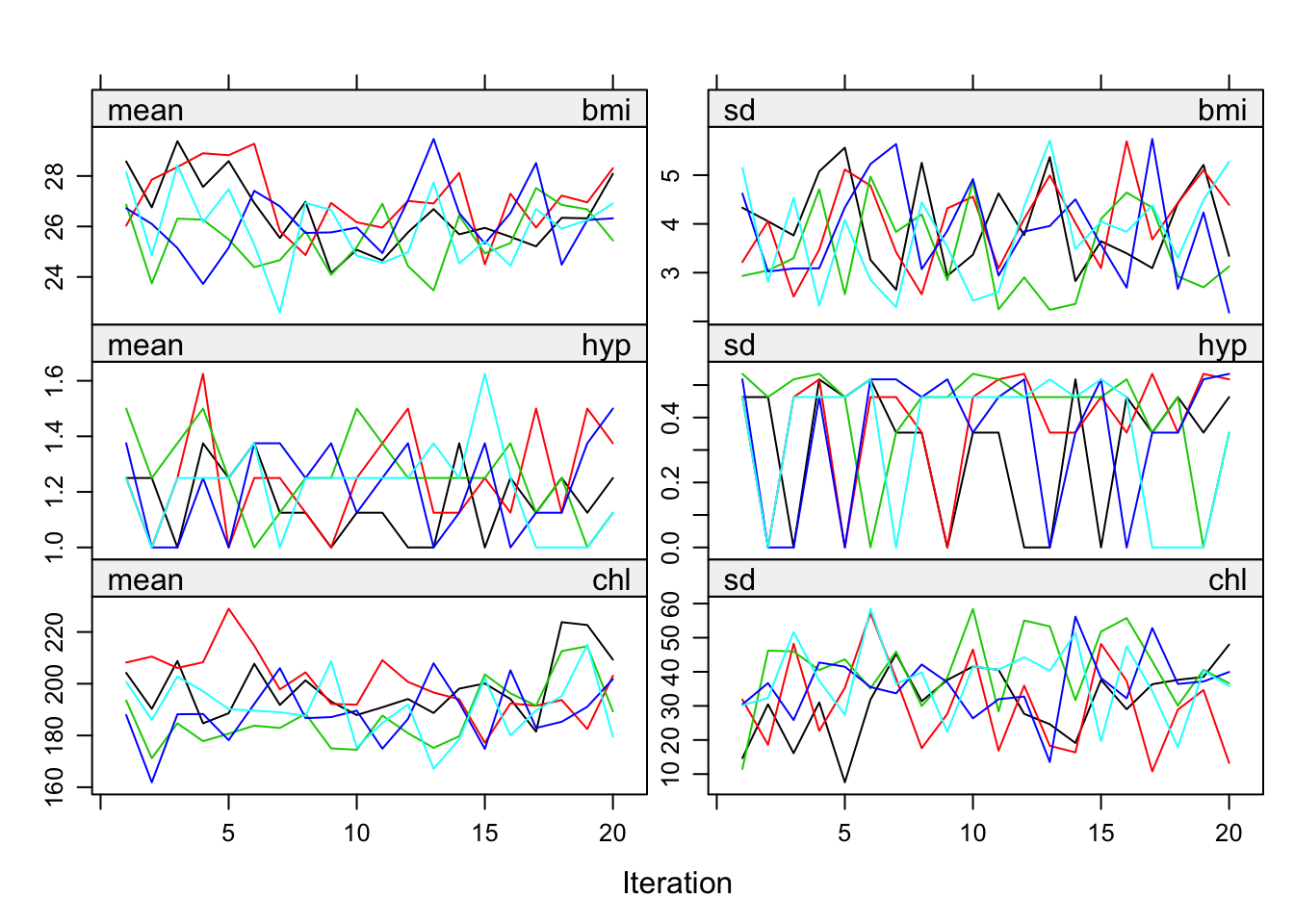
Figure 6.7: Mean and standard deviation of the synthetic values plotted against iteration number for the imputed nhanes data.

There is no clear-cut method for determining when the MICE algorithm has converged. It is useful to plot one or more parameters against the iteration number. The mean and variance of the imputations for each parallel stream can be plotted by

imp <- mice(nhanes, seed = 62006, maxit = 20, print = FALSE)
plot(imp)

which produces Figure 6.7. On convergence, the different streams should be freely intermingled with one another, without showing any definite trends. Convergence is diagnosed when the variance between different sequences is no larger than the variance within each individual sequence. Inspection of the streams may reveal particular problems of the imputation model. A pathological case of non-convergence occurs with the following code:

meth <- make.method(boys)
meth["bmi"] <- "~I(wgt / (hgt / 100)^2)"
imp.bmi1 <- mice(boys, meth = meth, maxit = 20,
                 print = FALSE, seed = 60109)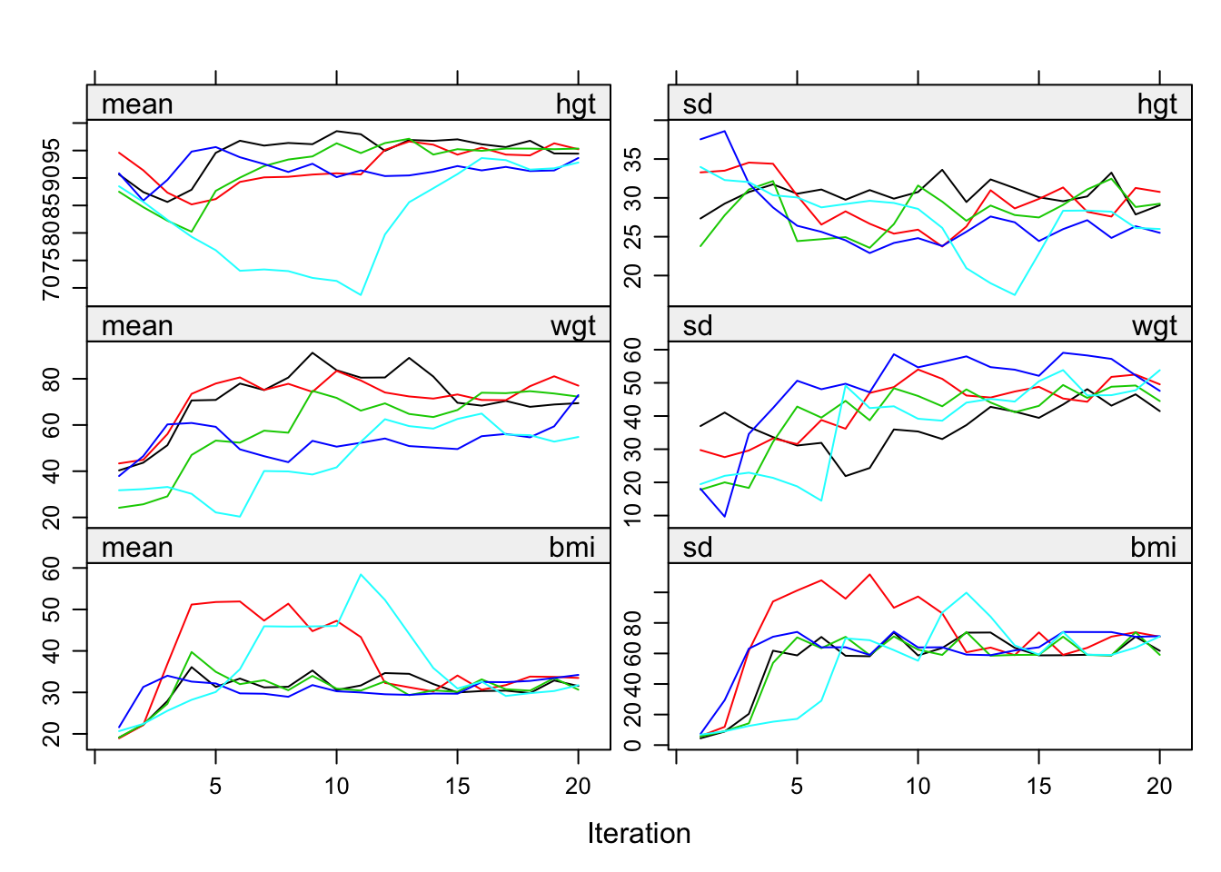

Figure 6.8: Non-convergence of the MICE algorithm caused by feedback of bmi into hgt and wgt.

Convergence is problematic here because imputations of bmi feed back into hgt and wgt. Figure 6.8 shows that the streams hardly mix and slowly resolve into a steady state. The problem is solved by breaking the feedback loop as follows:

pred <- make.predictorMatrix(boys)
pred[c("hgt", "wgt"), "bmi"] <- 0
imp.bmi2 <- mice(boys, meth = meth, pred = pred, maxit = 20,
                 print = FALSE, seed = 60109)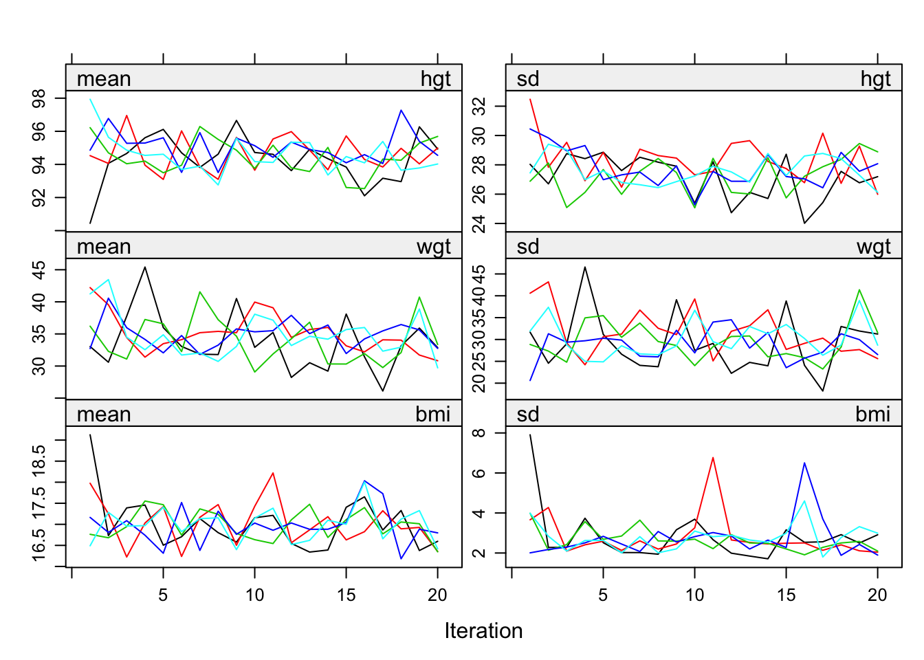

Figure 6.9: Healthy convergence of the MICE algorithm for hgt, wgt and bmi.

Figure 6.9 is the resulting plot for the same three variables. There is little trend and the streams mingle well.

The default plot() function for mids objects plots the mean and variance of the imputations. While these parameters are informative for the behavior of the MICE algorithm, they may not always be the parameter of greatest interest. It is easy to replace the mean and variance by other parameters, and monitor these. Schafer (1997, 129–31) suggested monitoring the “worst linear function” of the model parameters, i.e., a combination of parameters that will experience the most problematic convergence. If convergence can be established for this parameter, then it is likely that convergence will also be achieved for parameters that converge faster. Alternatively, we may monitor some statistic of scientific interest, e.g., a correlation or a proportion. See Sections 4.5.7 (Pearson correlation) and 9.4.3 (Kendall’s \(\tau\)) for examples.

It is possible to use formal convergence statistics. Several expository reviews are available that assess convergence diagnostics for MCMC methods (Cowles and Carlin 1996; Brooks and Gelman 1998; El Adlouni, Favre, and Bobée 2006). Cowles and Carlin (1996) conclude that “automated convergence monitoring (as by a machine) is unsafe and should be avoided.” No method works best in all circumstances. The consensus is to assess convergence with a combination of tools. The added value of using a combination of convergence diagnostics for missing data imputation has not yet been systematically studied.