3.2 Imputation under the normal linear normal

3.2.1 Overview

For univariate $Y$ we write lower-case $y$ for $Y$. Any predictors in the imputation model are collected in $X$. Symbol $X_\mathrm{obs}$ indicates the subset of $n_1$ rows of $X$ for which $y$ is observed, and $X_\mathrm{mis}$ is the complementing subset of $n_0$ rows of $X$ for which $y$ is missing. The vector containing the $n_1$ observed data in $y$ is denoted by $y_\mathrm{obs}$, and the vector of $n_0$ imputed values in $y$ is indicated by $\dot y$. This section reviews four different ways of creating imputations under the normal linear model. The four methods are:

Predict. $\dot y=\hat\beta_0+X_\mathrm{mis}\hat\beta_1$, where $\hat\beta_0$ and $\hat\beta_1$ are least squares estimates calculated from the observed data. Section 1.3.4 named this regression imputation. In mice this method is available as method norm.predict.
Predict + noise. $\dot y=\hat\beta_0+X_\mathrm{mis}\hat\beta_1+\dot\epsilon$, where $\dot\epsilon$ is randomly drawn from the normal distribution as $\dot\epsilon \sim N(0,\hat\sigma^2)$. Section 1.3.5 named this stochastic regression imputation. In mice this method is available as method norm.nob.
Bayesian multiple imputation. $\dot y =\dot\beta_0 + X_\mathrm{mis}\dot\beta_1+\dot\epsilon$, where $\dot\epsilon \sim N(0,\dot\sigma^2)$ and $\dot\beta_0$, $\dot\beta_1$ and $\dot\sigma$ are random draws from their posterior distribution, given the data. Section 3.1.3 named this “predict + noise + parameters uncertainty.” The method is available as method norm.
Bootstrap multiple imputation. $\dot y=\dot\beta_0+X_\mathrm{mis}\dot\beta_1+\dot\epsilon$, where $\dot\epsilon \sim N(0,\dot\sigma^2)$, and where $\dot\beta_0$, $\dot\beta_1$ and $\dot\sigma$ are the least squares estimates calculated from a bootstrap sample taken from the observed data. This is an alternative way to implement “predict + noise + parameters uncertainty.” The method is available as method norm.boot.

3.2.2 Algorithms$^\spadesuit$

The calculations of the first two methods are straightforward and do not need further explanation. This section describes the algorithms used to introduce sampling variability into the parameters estimates of the imputation model.

The Bayesian sampling draws $\dot\beta_0$, $\dot\beta_1$ and $\dot\sigma$ from their respective posterior distributions. Box and Tiao (1973 Section 2.7) explains the Bayesian theory behind the normal linear model. We use the method that draws imputations under the normal linear model using the standard noninformative priors for each of the parameters. Given these priors, the required inputs are:

$y_\mathrm{obs}$, the $n_1 \times 1$ vector of observed data in the incomplete (or target) variable $y$;
$X_\mathrm{obs}$, the $n_1 \times q$ matrix of predictors of rows with observed data in $y$;
$X_\mathrm{mis}$, the $n_0 \times q$ matrix of predictors of rows with missing data in $y$.

The algorithm assumes that both $X_\mathrm{obs}$ and $X_\mathrm{mis}$ contain no missing values. Chapter 4 deals with the case where $X_\mathrm{obs}$ and $X_\mathrm{mis}$ also could be incomplete.

Algorithm 3.1 (Bayesian imputation under the normal linear model.$^\spadesuit$)

Calculate the cross-product matrix $S=X_\mathrm{obs}^\prime X_\mathrm{obs}$.
Calculate $V = (S+\mathrm{diag}(S)\kappa)^{-1}$, with some small $\kappa$.
Calculate regression weights $\hat\beta = VX_\mathrm{obs}^\prime y_\mathrm{obs}$.
Draw a random variable $\dot g \sim \chi^2_\nu$ with $\nu=n_1 - q$.
Calculate $\dot\sigma^2 = (y_\mathrm{obs} - X_\mathrm{obs}\hat\beta)^\prime(y_\mathrm{obs} - X_\mathrm{obs}\hat\beta) / \dot g$.
Draw $q$ independent $N(0,1)$ variates in vector $\dot z_1$.
Calculate $V^{1/2}$ by Cholesky decomposition.
Calculate $\dot\beta = \hat\beta + \dot\sigma\dot z_1 V^{1/2}$.
Draw $n_0$ independent $N(0,1)$ variates in vector $\dot z_2$.
Calculate the $n_0$ values $y_\mathrm{imp} = X_\mathrm{mis}\dot\beta + \dot z_2\dot\sigma$.

Algorithm 3.1 is adapted from Rubin (1987 b, 167), and is implemented as the method norm (or, equivalently, as the function mice.impute.norm()) in the mice package. Any drawn values are identified with a dot above the symbol, so $\dot\beta$ is a value of $\beta$ drawn from the posterior distribution. The algorithm uses a ridge parameter $\kappa$ to evade problems with singular matrices. This number should be set to a positive number close to zero, e.g., $\kappa=0.0001$. For some data, larger $\kappa$ may be needed. High values of $\kappa$, e.g., $\kappa=0.1$, may introduce a systematic bias toward the null, and should thus be avoided.

Algorithm 3.2 (Imputation under the normal linear model with bootstrap.$^\spadesuit$)

Draw a bootstrap sample $(\dot y_\mathrm{obs},\dot X_\mathrm{obs})$ of size $n_1$ from $(y_\mathrm{obs},X_\mathrm{obs})$.}
Calculate the cross-product matrix $\dot S=\dot X_\mathrm{obs}^\prime\dot X_\mathrm{obs}$.
Calculate $\dot V = (\dot S+\mathrm{diag}(\dot S)\kappa)^{-1}$, with some small $\kappa$.
Calculate regression weights $\dot\beta = \dot V\dot X_\mathrm{obs}^\prime\dot y_\mathrm{obs}$.
Calculate $\dot\sigma^2 = (\dot y_\mathrm{obs} - \dot X_\mathrm{obs}\dot\beta)\prime(\dot y_\mathrm{obs} - \dot X_\mathrm{obs} \dot\beta)/(n_1-q-1)$.
Draw $n_0$ independent $N(0,1)$ variates in vector $\dot z_2$.
Calculate the $n_0$ values $y_\mathrm{imp} = X_\mathrm{mis}\dot\beta + \dot z_2\dot\sigma$.

The bootstrap is a general method for estimating sampling variability through resampling the data (Efron and Tibshirani 1993). Algorithm 3.2 calculates univariate imputations by drawing a bootstrap sample from the complete part of the data, and subsequently takes the least squares estimates given the bootstrap sample as a “draw” that incorporates sampling variability into the parameters (Heitjan and Little 1991). Compared to the Bayesian method, the bootstrap method avoids the Choleski decomposition and does not need to draw from the $\chi^2$-distribution.

3.2.3 Performance

Which of these four imputation methods of Section 3.2 is best? In order to find out let us conduct a small simulation experiment where we calculate the performance statistics introduced in Section 2.5.3. We keep close to the original data by assuming that $\beta_0=5.49$, $\beta_1= -0.29$ and $\sigma = 0.86$ are the population values. These values are used to generate artificial data with known properties.

Table 3.1: Properties of $\beta_1$ under imputation of missing $y$ by five methods for the normal linear model ($n_\mathrm{sim} = 10000$).
Method	Bias	Coverage	CI Width	RMSE
`norm.predict`	0.0000	0.652	0.114	0.063
`norm.nob`	-0.0001	0.908	0.226	0.064
`norm`	-0.0001	0.951	0.314	0.066
`norm.boot`	-0.0001	0.941	0.299	0.066
Listwise deletion	0.0001	0.946	0.251	0.063

Table 3.1 summarizes the results for the situation where we have 50% completely random missing in $y$ and $m = 5$. All methods are unbiased for $\beta_1$. The confidence interval of method norm.predict is much too short, leading to substantial undercoverage and $p$-values that are “too significant.” This result confirms the problems already noted in Section 2.6. The norm.nob method performs better, but the coverage of 0.908 is still too low. Methods norm and norm.boot and complete-case analysis are correct. Complete-case analysis is a correct analysis here (Little and Rubin 2002), and in fact the most efficient choice for this problem as it yields the shortest confidence interval (cf. Section 2.7). This result does not hold more generally. In realistic situations involving more covariates multiple imputation will rapidly catch up and pass complete-case analysis. Note that the RMSE values are uninformative for separating correct and incorrect methods, and are in fact misleading.

While method norm.predict is simple and fast, the variance estimate is too low. Several methods have been proposed to correct the estimate (Lee, Rancourt, and Särndal 1994; Fay 1996; Rao 1996; Schafer and Schenker 2000). Though such methods require special adaptation of formulas to calculate the variance, they may be useful when the missing data are restricted to the outcome.

Table 3.2: Properties of $\beta_1$ under imputation of missing $x$ by five methods for the normal linear model ($n_\mathrm{sim} = 10000$).
Method	Bias	% Bias	Coverage	CI Width	RMSE
`norm.predict`	-0.1007	34.7	0.359	0.160	0.118
`norm.nob`	0.0006	0.2	0.924	0.202	0.056
`norm`	0.0075	2.6	0.955	0.254	0.058
`norm.boot`	-0.0014	0.5	0.946	0.238	0.058
Listwise deletion	-0.0001	0.0	0.946	0.251	0.063

It is straightforward to adapt the simulations to other, perhaps more interesting situations. Investigating the effect of missing data in the explanatory $x$ instead of the outcome variable requires only a small change in the function to create the missing data. Table 3.2 displays the results. Method norm.predict is now severely biased, whereas the other methods remain unbiased. The confidence interval of norm.nob is still too short, but less than in Table 3.1. Methods norm, norm.boot and listwise deletion are correct, in the sense that these are unbiased and have appropriate coverage. Again, under the simulation conditions, listwise deletion is the optimal analysis. Note that norm is slightly biased, whereas method norm.boot slightly underestimates the variance. Both tendencies are small in magnitude. The RMSE values are uninformative, and are only shown to illustrate that point.

We could increase the number of explanatory variables and the number of imputations $m$ to see how much the average confidence interval width would shrink. It is also easy to apply more interesting missing data mechanisms, such as those discussed in Section 3.2.4. Data can be generated from skewed distributions, the sample size $n$ can be varied and so on. Extensive simulation work is available (Rubin and Schenker 1986 b; Rubin 1987 b).

3.2.4 Generating MAR missing data

Just making random missing data is not always interesting. We obtain more informative simulations if the missingness probability is a function of the observed, and possibly of the unobserved, information. This section considers some methods for creating missing data.

Let us first consider three methods to create missing data in artificial data. The data are generated as 1000 draws from the bivariate normal distribution $P(Y_1, Y_2)$ with means $\mu_1 = \mu_2 =5$, variances $\sigma_1^2 =\sigma_2^2 = 1$, and covariance $\sigma_{12} = 0.6$. We assume that all values generated are positive. Missing data in $Y_2$ can be created in many ways. Let $R_2$ be the response indicator for $Y_2$. We study three examples, each of which affects the distribution in different ways:

\[\begin{align} \mathrm{MARRIGHT} &:& \mathrm{logit}(\Pr(R_2=0)) = -5 + Y_1 \tag{3.1}\\ \mathrm{MARMID} &:& \mathrm{logit}(\Pr(R_2=0)) = 0.75 - |Y_1-5| \tag{3.2}\\ \mathrm{MARTAIL} &:& \mathrm{logit}(\Pr(R_2=0)) = -0.75 + |Y_1-5| \tag{3.3} \end{align}\]

where $\mathrm{logit}(p) = \log(p)-\log(1-p)$ with $0\leq p \leq 1$ is the logit function. Its inverse $\mathrm{logit}^{-1}(x) = \exp(x)/(1+\exp(x))$ is known as the logistic function.

Generating missing data under these models in R can be done in three steps: calculate the missingness probability of each data point, make a random draw from the binomial distribution and set the corresponding observations to NA. The following script creates missing data according to MARRIGHT:

set.seed(1)
n <- 10000
sigma <- matrix(c(1, 0.6, 0.6, 1), nrow = 2)
cmp <- MASS::mvrnorm(n = n, mu = c(5, 5), Sigma = sigma)
p2.marright <- 1 - plogis(-5 + cmp[, 1])
r2.marright <- rbinom(n, 1, p2.marright)
yobs <- cmp
yobs[r2.marright == 0, 2] <- NA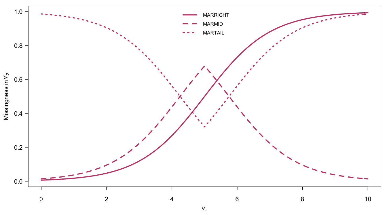

$Probability that $Y_2$ is missing as a function of the values of $Y_1$ under three models for the missing data.$

Figure 3.2: Probability that $Y_2$ is missing as a function of the values of $Y_1$ under three models for the missing data.

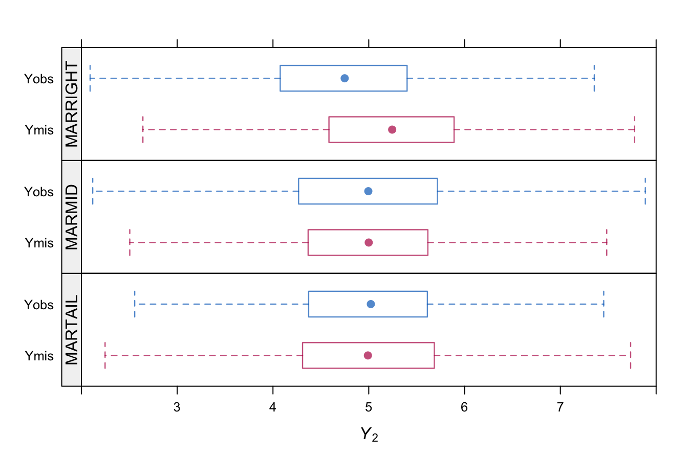
$Box plot of $Y_2$ separated for the observed and missing parts under three models for the missing data based on $n=10000$.$

Figure 3.3: Box plot of $Y_2$ separated for the observed and missing parts under three models for the missing data based on $n=10000$.

Figure 3.2 displays the probability of being missing under the three MAR mechanisms. All mechanisms yield approximately 50% of missing data, but do so in very different ways. Figure 3.3 displays the distributions of $Y_2$ under the three models. MARRIGHT deletes more high values, so the distribution of the observed data shifts to the left. MARMID deletes more data in the center, so the variance of the observed data grows, but the mean is not affected. MARTAIL shows the reverse effect. The variance of observed data reduces because the missing data occur in the tails.

These mechanisms are more extreme than we are likely to see in practice. Not only is there a strong relation between $Y_1$ and $R_2$, but the percentage of missing data is also quite high (50%). On the other hand, if methods perform well under these data deletion schemes, they will also do so in less extreme situations that are more likely to be encountered in practice.

3.2.5 MAR missing data generation in multivariate data

Creating missing data from complete data is easy to do for simple scenarios with one missing value per row. Things become more complicated for multiple missing values per unit, as we need to be careful not to delete any values that are needed to make the problem MAR.

Brand (1999, 110–13) developed the following method for generating non-monotone multivariate missing data in $p$ variables $Y_1,\dots,Y_p$. We assume that $Y=(Y_1,\dots,Y_p)$ is initially completely known. The method requires specification of

$\alpha$, the desired proportion of incomplete cases,
$R_\mathrm{pat}$, a binary $n_\mathrm{pat} \times p$ matrix defining $n_\mathrm{pat}$ allowed patterns of missing data, where all response patterns except $(0,0,\dots,0)$ and $(1,1,\dots,1)$ may occur,
$f=(f_{(1)},\dots,f_{(n_\mathrm{pat})})$, a vector containing the relative frequencies of each pattern, scaled such that $\sum_{s}^{n_\mathrm{pat}} f_{(s)} = 1$,
$P(R|Y)=(P(R_{(1)}|Y{(1)}),\dots,P(R_{(n_\mathrm{pat})}|Y_{(n_\mathrm{pat})}))$, a set of $n_\mathrm{pat}$ response probability models, one for each pattern.

The general procedure is as follows: Each case is allocated to one of $n_\mathrm{pat}$ candidate blocks using a random draw from the multinomial distribution with probabilities $f_{(1)},\dots,f_{(n_\mathrm{pat})}$. Within the $s^\mathrm{th}$ candidate block, a subgroup of $\alpha nf_{(s)}$ cases is made incomplete according to pattern $R_{(s)}$ using the missing data model $P(R_{(s)}|Y_{(s)})$, where $s=1,\dots,n_\mathrm{pat}$. The procedure results in approximately $\alpha$ incomplete cases, that are distributed over the allowed response patterns. If the missing data are to be MAR, then the missing variables in the $s^\mathrm{th}$ pattern should not influence the missingness probability defined by the missing data model $P(R_{(s)}|Y_{(s)}$ for block $s$.

The ampute() function in mice implements the method. For example, we can create 50% missing data in both $Y_1$ and $Y_2$ according to a MARRIGHT scenario by

amp <- ampute(cmp, type = "RIGHT")
apply(amp$amp, 2, mean, na.rm = TRUE)

  V1   V2 
4.91 4.91

As expected, the means in the amputed data are lower than in the complete data. It is possible to inspect the distributions of the observed data more closely by md.pattern(amp$amp), bwplot(amp) and xyplot(amp). Many options are available that allows the user to tailor the missing data patterns to the data at hand. See Schouten, Lugtig, and Vink (2018) for details.

3.2.6 Conclusion

Tables 3.1 and 3.2 show that methods norm.predict (regression imputation) and norm.nob (stochastic regression imputation) fail in terms of understating the uncertainty in the imputations. If the missing data occur in $y$ only, then it is possible to correct the variance formulas of method norm.predict. However, if the missing data occur in $X$, norm.predict is severely biased, so then variance correction is not useful. Methods norm and norm.boot account for the uncertainty of the imputation model provide statistically correct inferences. For missing $y$, the efficiency of these methods is less than theoretically possible, presumably due to simulation error.

It is always better to include parameter uncertainty, either by the Bayesian or the bootstrap method. The effect of doing so will diminish with increasing sample size (Exercise 3.2), so for estimates based on a large sample one may opt for the simpler norm.nob method if speed of calculation is at premium. Note that in subgroup analyses, the large-sample requirement applies to the subgroup size, and not to the total sample size.