4.6 FCS and JM

4.6.1 Relations between FCS and JM

FCS is related to JM in some special cases. If \(P(X, Y)\) has a multivariate normal model distribution, then all conditional densities are linear regressions with a constant normal error variance. So, if \(P(X, Y)\) is multivariate normal then \(P(Y_j | X, Y_{-j})\) follows a linear regression model. The reverse is also true: If the imputation models \(P(Y_j | X, Y_{-j})\) are all linear with constant normal error variance, then the joint distribution will be multivariate normal. See Arnold, Castillo, and Sarabia (1999, 186) for a description of the precise conditions. Thus, imputation by FCS using all linear regressions is identical to imputation under the multivariate normal model.

Another special case occurs for binary variables with only two-way interactions in the log-linear model. In the special case \(p=3\) suppose that \(Y_1,\dots,Y_3\) are modeled by the log-linear model that has the three-way interaction term set to zero. It is known that the corresponding conditional distribution \(P(Y_1|Y_2,Y_3)\) is the logistic regression model \(\log(P(Y_1)/1-P(Y_1)) = \beta_0 + \beta_2Y_2 + \beta_3Y_3\) (Goodman 1970). Analogous definitions exist for \(P(Y_2|Y_1,Y_3)\) and \(P(Y_3|Y_1,Y_2)\). This means that if we use logistic regressions for \(Y_1\), \(Y_2\) and \(Y_3\), we are effectively imputing under the multivariate “no three-way interaction” log-linear model. Hughes et al. (2014) showed that this relation does not extend to more than three variables.

4.6.2 Comparisons

FCS cannot use computational shortcuts like the sweep operator, so the calculations per iterations are more intensive than under JM. Also, JM has better theoretical underpinnings.

On the other hand, FCS allows tremendous flexibility in creating multivariate models. One can easily specify models that are outside any known standard multivariate density \(P(X, Y, R|\theta)\). FCS can use specialized imputation methods that are difficult to formulate as a part of a multivariate density \(P(X, Y, R |\theta)\). Imputation methods that preserve unique features in the data, e.g., bounds, skip patterns, interactions, bracketed responses and so on can be incorporated. It is possible to maintain constraints between different variables in order to avoid logical inconsistencies in the imputed data that would be difficult to do as part of a multivariate density \(P(X, Y, R |\theta)\).

Lee and Carlin (2010) found that JM performs as well as FCS, even in the presence of binary and ordinal variables. These authors also observed substantial improvements for skewed variables by transforming the variable to symmetry (for JM) or by using predictive mean matching (for FCS). Kropko et al. (2014) found that JM and FCS performed about equally well for continuous and binary variable, but FCS outperforms JM on every metric when the variable of interest is categorical. With predictive mean matching, FCS outperforms JM “for every metric and variable type, including the continuous variable.” Seaman and Hughes (2018) compared FCS to a restricted general location model. As expected, the latter model is more efficient when correctly specified, but the gains are small unless the relations between the variables are very strong. As FCS was found to be more robust under misspecification, the authors advise FCS over JM.

4.6.3 Illustration

The Fourth Dutch Growth Study by Fredriks, Van Buuren, Burgmeijer, et al. (2000) collected data on 14500 Dutch children between 0 and 21 years. The development of secondary pubertal characteristics was measured by the so-called Tanner stages, which divides the continuous process of maturation into discrete stages for the ages between 8 and 21 years. Pubertal stages of boys are defined for genital development (gen: five ordered stages G1–G5), pubic hair development (phb: six ordered stages P1–P6) and testicular volume (tv: 1–25ml).

We analyze the subsample of 424 boys in the age range 8–21years using the boys data in mice. There were 180 boys (42%) for which scores for genital development were missing. The missingness was strongly related to age, rising from about 20% at ages 9–11 years to 60% missing data at ages 17–20 years.

The data consist of three complete covariates: age (age), height (hgt) and weight (wgt), and three incomplete outcomes measuring maturation. The following code block creates \(m = 10\) imputations by the normal model, by predictive mean matching and by the proportional odds model.

select <- with(boys, age >= 8 & age <= 21.0)
djm <- boys[select, -4]
djm$gen <- as.integer(djm$gen)
djm$phb <- as.integer(djm$phb)
djm$reg <- as.integer(djm$reg)
dfcs <- boys[select, -4]

## impute under jm and fcs
jm <- mice(djm, method = "norm", seed = 93005, m = 10,
           print = FALSE)
pmm <- mice(djm, method = "pmm", seed = 71332, m = 10,
            print = FALSE)
fcs <- mice(dfcs, seed = 81420, m = 10, print = FALSE)

Figure 4.4 plots the results of the first five imputations from the normal model. It was created by the following statement:

xyplot(jm, gen ~ age | as.factor(.imp), subset = .imp < 6,
       xlab = "Age", ylab = "Genital stage", col = mdc(1:2),
       ylim = c(0, 6))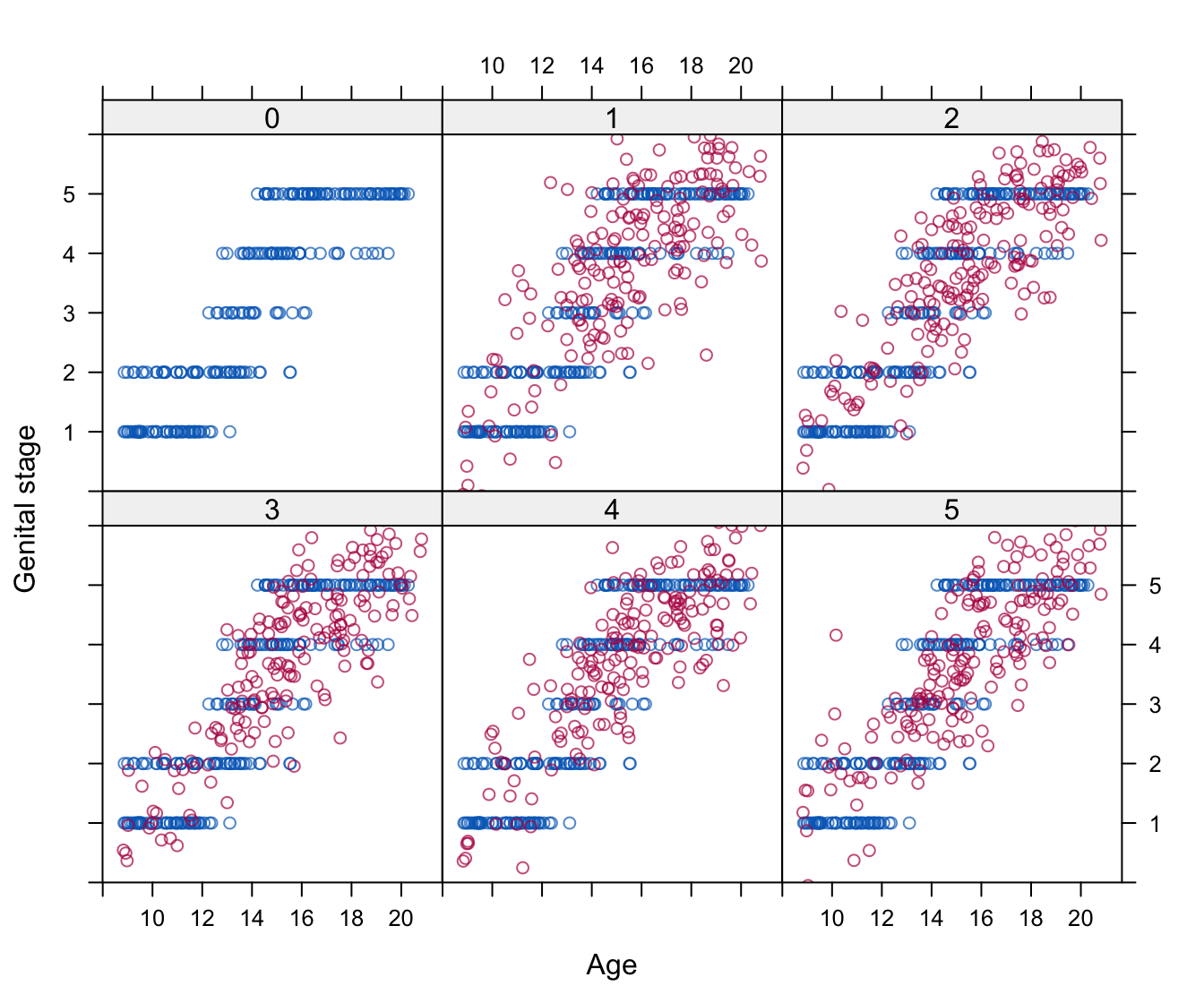

Figure 4.4: Joint modeling: Imputed data for genital development (Tanner stages G1–G5) under the multivariate normal model. The panels are labeled by the imputation numbers 0–5, where 0 is the observed data and 1–5 are five multiply imputed datasets.

The figure portrays how genital development depends on age for both the observed and imputed data. The spread of the synthetic values in Figure 4.4 is larger than the observed data range. The observed data are categorical while the synthetic data vary continuously. Note that there are some negative values in the imputations. If we are to do categorical data analysis on the imputed data, we need some form of rounding to make the synthetic values comparable with the observed values.

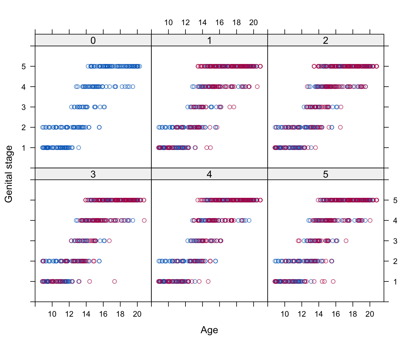
Figure 4.5: Fully conditional specification: Imputed data of genital development (Tanner stages G1–G5) under the proportional odds model.

Imputations for the proportonal odds model in Figure 4.5 differ markedly from those in Figure 4.4. This model yields imputations that are categorical, and hence no rounding is needed.

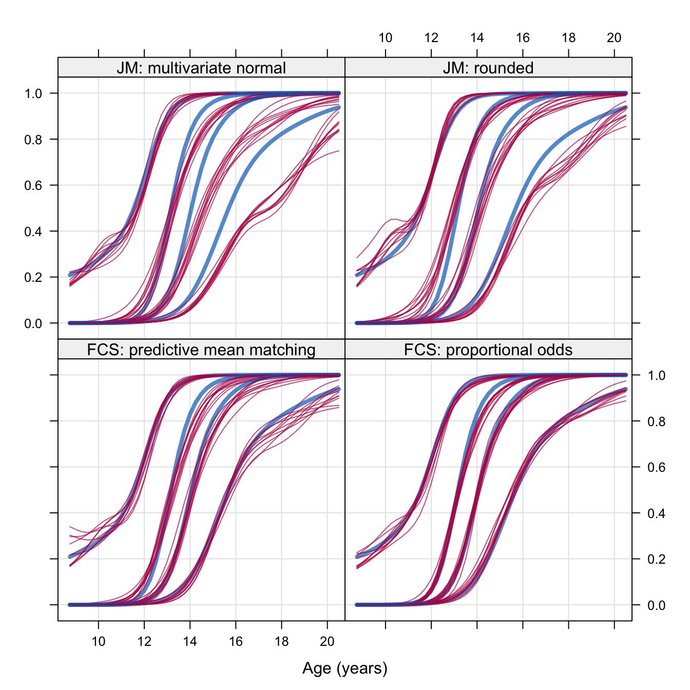
Figure 4.6: Probability of achieving stages G2–G5 of genital developmental by age (in years) under four imputation methods (\(m=10\)).

The complete-data model describes the probability of achieving each Tanner stage as a nonlinear function of age according to the model proposed in Van Buuren and Ooms (2009). The calculations are done with gamlss (Stasinopoulos and Rigby 2007). Under the assumption of ignorability, analysis of the complete cases will not be biased, so the complete-case analysis provides a handle to the appropriate solution. The blue lines in Figure 4.6 indicate the model fitted on the complete cases, whereas the thin black lines correspond to the analyses of the 10 imputed datasets.

The different panels of Figure 4.6 corresponds to different imputation methods. The panel labeled JM: multivariate normal contains the model fitted to the unprocessed imputed data produced under the multivariate normal model. There is a large discrepancy between the complete-case analysis and the models fitted to the imputed data, especially for the older boys. The fit improves in the panel labeled JM: rounded, where imputed data are rounded to the nearest category. There is considerable misfit, and the behavior of the imputed data around the age of 10years is a bit curious. The panel labeled FCS: predictive mean matching applied Algorithm 3.3 as a component of the MICE algorithm. Though this technique improves upon the previous two methods, some discrepancies for the older boys remain. The panel labeled FCS: proportional odds displays the results after applying the method for ordered categorical data as discussed in Section 3.6. The imputed data essentially agree with the complete-case analysis, perhaps apart from some minor deviations around the probability level of 0.9.

Figure 4.6 shows clear differences between FCS and JM when data are categorical. Although rounding may provide reasonable results in particular datasets, it seems that it does more harm than good here. There are many ways to round, rounding may require unrealistic assumptions and it will attenuate correlations. Horton, Lipsitz, and Parzen (2003), Ake (2005) and Allison (2005) recommend against rounding when data are categorical. See Section 4.4.3. Horton, Lipsitz, and Parzen (2003) expected that bias problems of rounding would taper off if variables have more than two categories, but the analysis in this section suggests that JM may also be biased for categorical data with more than two categories. Even though it may sound a bit trivial, my recommendation is: Impute categorical data by methods for categorical data.