6.3 Model form and predictors

6.3.1 Model form

The MICE algorithm requires a specification of a univariate imputation method separately for each incomplete variable. Chapter 3 discussed many possible methods. The measurement level largely determines the form of the univariate imputation model. The mice() function distinguishes numerical, binary, ordered and unordered categorical data, and sets the defaults accordingly.

Table 6.1: Built-in univariate imputation techniques in the mice package. Methods marked by \(^*\) are default for scale type.

Method	Description	Scale Type
pmm	Predictive mean matching	Any\(^*\)
midastouch	Weighted predictive mean matching	Any
sample	Random sample from observed values	Any
cart	Classification and regression trees	Any
rf	Random forest imputation	Any
mean	Unconditional mean imputation	Numeric
norm	Bayesian linear regression	Numeric
norm.boot	Normal imputation with bootstrap	Numeric
norm.nob	Normal imputation ignoring model error	Numeric
norm.predict	Normal imputation, predicted values	Numeric
quadratic	Imputation of quadratic terms	Numeric
ri	Random indicator for nonignorable data	Numeric
logreg	Logistic regression	Binary\(^*\)
logreg.boot	Logistic regression with bootstrap	Binary
polr	Proportional odds model	Ordinal\(^*\)
polyreg	Polytomous logistic regression	Nominal\(^*\)
lda	Discriminant analysis	Nominal

Table 6.1 lists the built-in univariate imputation method in the mice package. The defaults have been chosen to work well in a wide variety of situations, but in particular cases different methods may be better. For example, if it is known that the variable is close to normally distributed, using norm instead of the default pmm may be more efficient. For large datasets where sampling variance is not an issue, it could be useful to select norm.nob, which does not draw regression parameters, and is thus simpler and faster. The norm.boot method is a fast non-Bayesian alternative for norm. The norm methods are an alternative to pmm in cases where pmm does not work well, e.g., when insufficient nearby donors can be found.

The mean method is included for completeness and should not be generally used. For sparse categorical data, it may be better to use method pmm instead of logreg, polr or polyreg. Method logreg.boot is a version of logreg that uses the bootstrap to emulate sampling variance. Method lda is generally inferior to polyreg (Brand 1999), and should be used only as a backup when all else fails. Finally, sample is a quick method for creating starting imputations without the need for covariates.

6.3.2 Predictors

A useful feature of the mice() function is the ability to specify the set of predictors to be used for each incomplete variable. The basic specification is made through the predictorMatrix argument, which is a square matrix of size ncol(data) containing 0/1 data. Each row in predictorMatrix identifies which predictors are to be used for the variable in the row name. If diagnostics = TRUE (the default), then mice() returns a mids object containing a predictorMatrix entry. For example, type

imp <- mice(nhanes, print = FALSE)
imp$predictorMatrix

    age bmi hyp chl
age   0   1   1   1
bmi   1   0   1   1
hyp   1   1   0   1
chl   1   1   1   0

The rows correspond to incomplete target variables, in the sequence as they appear in the data. A value of 1 indicates that the column variable is a predictor to impute the target (row) variable, and a 0 means that it is not used. Thus, in the above example, bmi is predicted from age, hyp and chl. Note that the diagonal is 0 since a variable cannot predict itself. Since age contains no missing data, mice() silently sets all values in the row to 0. The default setting of the predictorMatrix specifies that every variable predicts all others.

Conditioning on all other data is often reasonable for small to medium datasets, containing up to, say, 20–30 variables, without derived variables, interactions effects and other complexities. As a general rule, using every bit of available information yields multiple imputations that have minimal bias and maximal efficiency (Meng 1994; Collins, Schafer, and Kam 2001). It is often beneficial to choose as large a number of predictors as possible. Including as many predictors as possible tends to make the MAR assumption more plausible, thus reducing the need to make special adjustments for MNAR mechanisms (Schafer 1997).

For datasets containing hundreds or thousands of variables, using all predictors may not be feasible (because of multicollinearity and computational problems) to include all these variables. It is also not necessary. In my experience, the increase in explained variance in linear regression is typically negligible after the best, say, 15 variables have been included. For imputation purposes, it is expedient to select a suitable subset of data that contains no more than 15 to 25 variables. provide the following strategy for selecting predictor variables from a large database:

1. Include all variables that appear in the complete-data model, i.e., the model that will be applied to the data after imputation, including the outcome (Little 1992; Moons et al. 2006). Failure to do so may bias the complete-data model, especially if the complete-data model contains strong predictive relations. Note that this step is somewhat counter-intuitive, as it may seem that imputation would artificially strengthen the relations of the complete-data model, which would be clearly undesirable. If done properly however, this is not the case. On the contrary, not including the complete-data model variables will tend to bias the results toward zero. Note that interactions of scientific interest also need to be included in the imputation model.

2. In addition, include the variables that are related to the nonresponse. Factors that are known to have influenced the occurrence of missing data (stratification, reasons for nonresponse) are to be included on substantive grounds. Other variables of interest are those for which the distributions differ between the response and nonresponse groups. These can be found by inspecting their correlations with the response indicator of the variable to be imputed. If the magnitude of this correlation exceeds a certain level, then the variable should be included.

3. In addition, include variables that explain a considerable amount of variance. Such predictors help reduce the uncertainty of the imputations. They are basically identified by their correlation with the target variable.

4. Remove from the variables selected in steps 2 and 3 those variables that have too many missing values within the subgroup of incomplete cases. A simple indicator is the percentage of observed cases within this subgroup, the percentage of usable cases (cf. Section 4.1.2).

Most predictors used for imputation are incomplete themselves. In principle, one could apply the above modeling steps for each incomplete predictor in turn, but this may lead to a cascade of auxiliary imputation problems. In doing so, one runs the risk that every variable needs to be included after all.

In practice, there is often a small set of key variables, for which imputations are needed, which suggests that steps 1 through 4 are to be performed for key variables only. This was the approach taken in Van Buuren and Groothuis-Oudshoorn (1999), but it may miss important predictors of predictors. A safer and more efficient, though more laborious, strategy is to perform the modeling steps also for the predictors of predictors of key variables. This is done in Groothuis-Oudshoorn, Van Buuren, and Van Rijckevorsel (1999). I expect that it is rarely necessary to go beyond predictors of predictors. At the terminal node, we can apply a simple method like sample that does not need any predictors for itself.

The mice package contains several tools that aid in automatic predictor selection. The quickpred() function is a quick way to define the predictor matrix using the strategy outlined above. The flux() function was introduced in Section 4.1.3. The mice() function detects multicollinearity, and solves the problem by removing one or more predictors for the model. Each removal is noted in the loggedEvents element of the mids object. For example,

imp <- mice(cbind(nhanes, chl2 = 2 * nhanes$chl),
            print = FALSE, maxit = 1, m = 3, seed = 1)

Warning: Number of logged events: 1

imp$loggedEvents

  it im dep      meth  out
1  0  0     collinear chl2

yields a warning that informs us that at initialization variable chl2 was removed from the imputation model because it is collinear with chl. As a result, chl will be imputed, but chl2 is not. We may override removal by

imp <- mice(cbind(nhanes, chl2 = 2 * nhanes$chl),
            print = FALSE, maxit = 1, m = 3, seed = 1,
            remove.collinear = FALSE)

Warning: Number of logged events: 3

imp$loggedEvents

  it im  dep meth out
1  1  1 chl2  pmm chl
2  1  2 chl2  pmm chl
3  1  3 chl2  pmm chl

Now, the algorithm detects multicollinearity during iterations, and removes chl from the imputation model for chl2. Although this imputes both chl and chl2, their relation is not maintained. See Figure 6.1.

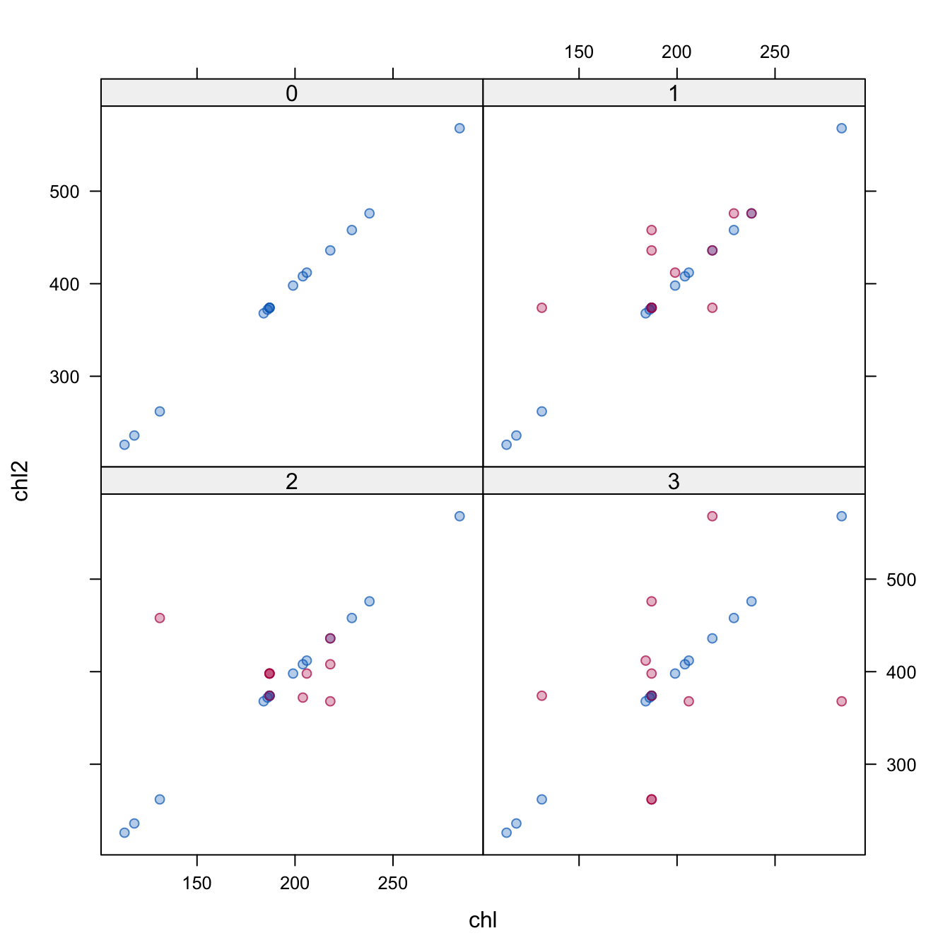
Figure 6.1: Scatterplot of chl2 against chl for \(m = 3\). The observed data are linearly related, but the imputed data do not respect the relationship.

As a general rule, feedback between different versions of the same variable should be prevented. The next section describes a number of techniques that are useful in various situations. Another measure to control the algorithm is the ridge parameter, denoted by \(\kappa\) in Algorithms 3.1, 3.2 and 3.3. The ridge parameter is specified as an argument to mice(). Setting ridge=0.001 or ridge=0.01 makes the algorithm more robust at the expense of bias.