9.4 Enhancing comparability

9.4.1 Description of the problem

Comparability of data is a key problem in international comparisons and meta analysis. The problem of comparability has many sides. An overview of the issues and methodologies can be found in Van Deth (1998), Harkness, Van de Vijver, and Mohler (2002), Salomon, Tandon, and Murray (2004), King et al. (2004), Matsumoto and Van de Vijver (2010) and Chevalier and Fielding (2011).

This section addresses just one aspect, incomparability of the data obtained on survey items with different questions or response categories. This is a very common problem that hampers many comparisons.

One of the tasks of the European Commission is to provide insight into the level of disability of the populations in each of the 27 member states of the European Union. Many member states conduct health surveys, but the precise way in which disability is measured are very different. For example, The U.K. Health Survey contains a question How far can you walk without stopping/experiencing severe discomfort, on your own, with aid if normally used? with response categories “can’t walk,” “a few steps only,” “more than a few steps but less than 200 yards” and “200 yards or more.” The Dutch Health Interview Survey contains the question Can you walk 400 metres without resting (with walking stick if necessary)? with response categories “yes, no difficulty,” “yes, with minor difficulty,” “yes, with major difficulty” and “no.” Both items obviously intend to measure the ability to walk, but it is far from clear how an answer on the U.K. item can be compared with one on the Dutch item.

Response conversion (Van Buuren et al. 2005) is a way to solve this problem. The technique transforms responses obtained on different questions onto a common scale. Where this can be done, comparisons can be made using the common scale. The actual data transformation can be repeatedly done on a routine basis as new information arrives. The construction of conversion keys is only possible if enough overlapping information can be identified. Keys have been constructed for dressing disability (Van Buuren et al. 2003), personal care disability, sensory functioning and communication, physical well-being (Van Buuren and Tennant 2004), walking disability (Van Buuren et al. 2005) and physical activity (Hopman-Rock et al. 2012).

This section presents an extension based on multiple imputation. The approach is more flexible and more general than response conversion. Multiple imputation does not require a common items into each other, whereas response conversion scales the data on a common scale. Multiple imputation does not require a common unidimensional latent scale, thereby increasing the range of applications.

9.4.2 Full dependence: Simple equating

In principle, the comparability problem is easy to solve if all sources would collect the same data. In practice, setting up and maintaining a centralized, harmonized data collection is easier said than done. Moreover, even where such efforts are successful, comparability is certainly not guaranteed (Harkness, Van de Vijver, and Mohler 2002). Many factors contribute to the incomparability of data, but we will not go into details here.

In the remainder, we take an example of two bureaus that each collect health data on its own population. The bureaus use survey items that are similar, but not the same. The survey used by bureau A contains an item for measuring walking disability (item A):

Are you able to walk outdoors on flat ground?

1. Without any difficulty

2. With some difficulty

3. With much difficulty

4. Unable to do

The frequencies observed in sample A are 242, 43, 15 and 0. There are six missing values. Bureau A produces a yearly report containing an estimate of the mean of the distribution of population A on item A. Assuming MCAR, a simple random sample and equal inter-category distances, we find \(\hat\theta_\mathrm{AA}\) = (242 \(\times\) 0 + 43 \(\times\) 1 + 15 \(\times\) 2) / 300 = 0.243, the disability estimate for population A using the method of bureau A.

The survey of bureau B contains item B:

Can you, fully independently, walk outdoors (if necessary, with a cane)?

1. Yes, no difficulty

2. Yes, with some difficulty

3. Yes, with much difficulty

4. No, only with help from others

The frequencies observed in sample B are 145, 110, 29 and 8. There were no missing values reported by bureau B. Bureau B publishes the proportion of cases in category 0 as a yearly health measure. Assuming a simple random sample, \(P(Y_\mathrm{B}=0)\) is estimated by \(\hat\theta_\mathrm{BB}\) = 145 / 292 = 0.497, the health estimate for population B using the method of bureau B.

Note that \(\hat\theta_\mathrm{AA}\) and \(\hat\theta_\mathrm{BB}\) are different statistics calculated on different samples, and hence cannot be compared. On the surface, the problem is trivial and can be solved by just equating the four categories. After that is done, and we can apply the methods of bureau A or B, and compare the results. Such recoding to “make data comparable” is widely practiced.

Let us calculate the result using simple equating. To estimate walking disability in population B using the method of bureau A we obtain \(\hat\theta_\mathrm{BA}\) = (145 \(\times\) 0 + 110 \(\times\) 1 + 29 \(\times\) 2 + 8 \(\times\) 3) / 292 = 0.658. Remember that the mean disability estimate for population A was equal to 0.243, so population B appears to have substantially more walking disability. The difference equals \(\hat\theta_\mathrm{BA} - \hat\theta_\mathrm{AA}\) = 0.658 - 0.243 = 0.414 on a scale from 0 to 3.

Likewise, we may estimate bureau’s B health measure \(\theta_\mathrm{AB}\) in population A as \(\hat\theta_\mathrm{AB}\) = 242 / 300 = 0.807. Thus, over 80% of population A scores in category 0. This is substantially more than in population B, which was \(\hat\theta_\mathrm{BB}\) = 145/292 = 0.497.

So by equating categories both bureaus conclude that the healthier population is A, and by a fairly large margin. As we will see, this result is however highly dependent on assumptions that may not be realistic for these data.

9.4.3 Independence: Imputation without a bridge study

Let \(Y_\mathrm{A}\) be the item of bureau A, and let \(Y_\mathrm{B}\) be the item of bureau B. The comparability problem can be seen as a missing data problem, where \(Y_\mathrm{A}\) is missing for population B, and where \(Y_\mathrm{B}\) is missing for population A. This formulation suggest that we can use imputation to solve the problem, and calculate \(\hat\theta_\mathrm{AB}\) and \(\hat\theta_\mathrm{BA}\) from the imputed data.

Let’s see what happens if we put mice() to work to solve the problem. We first create the dataset:

fA <- c(242, 43, 15, 0, 6)
fB <- c(145, 110, 29, 8)
YA <- rep(ordered(c(0:3, NA)), fA)
YB <- rep(ordered(c(0:3)), fB)
Y <- rbind(data.frame(YA, YB = ordered(NA)),
           data.frame(YB, YA = ordered(NA)))

Figure 9.7: Missing data pattern for walking data without a bridge study.

The data Y is a data frame with 604 rows and 2 columns: YA and YB. Figure ?? shows that the missing data pattern is unconnected (cf. Section 4.1.1), with no observations linking YA to YB. There are six records that contain no data at all.

For this problem, we monitor the behavior of a rank-order correlation, facility in mice(), but we can easily write a small function micemill() that calculates Kendall’s \(\tau\) after each iteration as follows.

ra <- function(x, simplify = FALSE) {
  if (!is.mira(x)) return(NULL)
  ra <- x$analyses
  if (simplify) ra <- unlist(ra)
  return(ra)
}
micemill <- function(n) {
  for (i in 1:n) {
    imp <<- mice.mids(imp, print = FALSE)
    cors <- with(imp, cor(as.numeric(YA), as.numeric(YB),
                          method = "kendall"))
    tau <<- rbind(tau, ra(cors, simplify = TRUE))
  }
}

This function calls mice.mids() to perform just one iteration, calculates Kendall’s \(\tau\), and stores the result. Note that the function contains two double assignment operators. This allows the function to overwrite the current imp and tau object in the global environment. This is a dangerous operation, and not really an example of good programming in general. However, we may now write

tau <- NULL
imp <- mice(Y, maxit = 0, m = 10, seed = 32662, print = FALSE)
micemill(50)

This code executes 50 iterations of the MICE algorithm. After any number of iterations, we may plot the trace lines of the MICE algorithm by

plotit <- function()
  matplot(x = 1:nrow(tau), y = tau,
          ylab = expression(paste("Kendall's ", tau)),
          xlab = "Iteration", type = "l", las = 1)
plotit()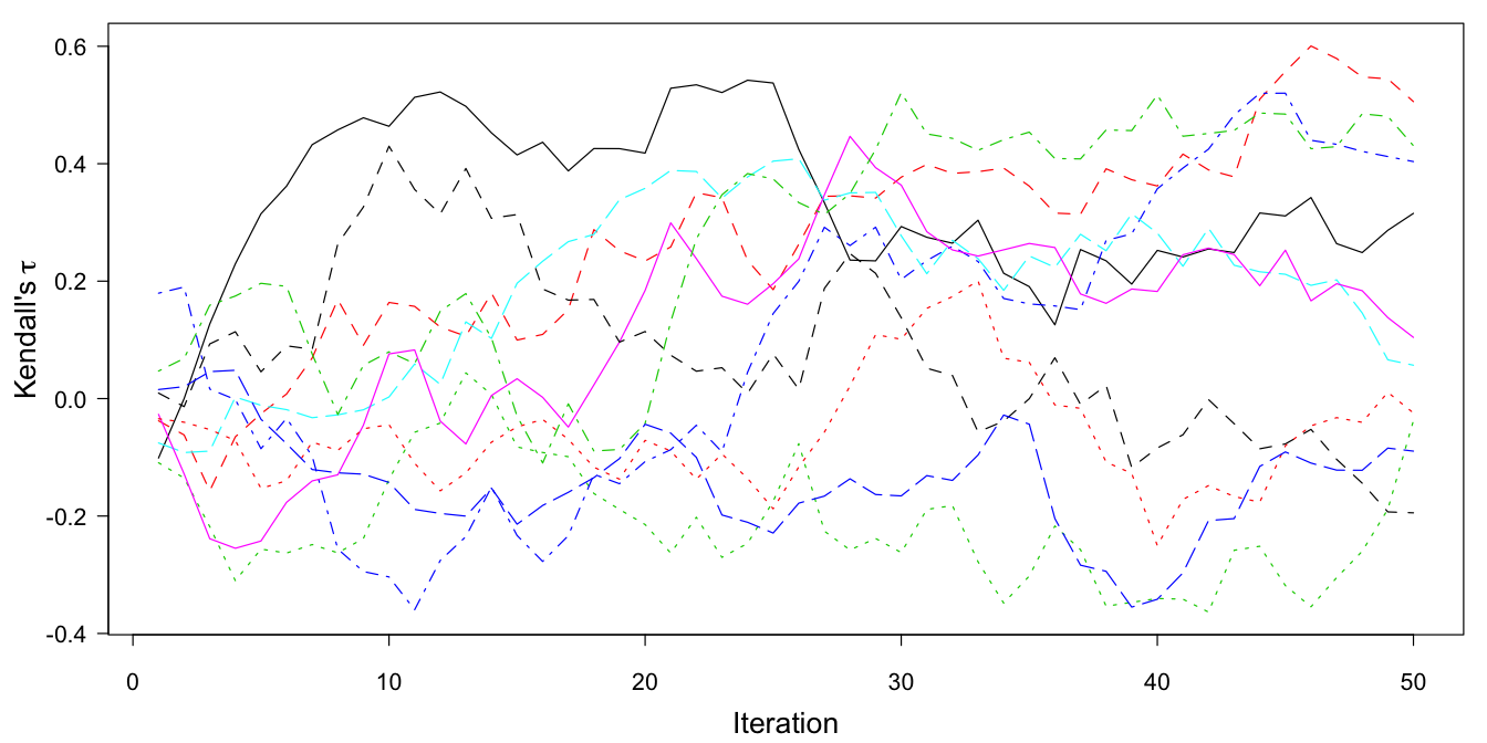

Figure 9.8: The trace plot of Kendall’s \(\tau\) for \(Y_\mathrm{A}\) and \(Y_\mathrm{B}\) using \(m=10\) multiple imputations and 50 iterations. The data contain no cases that have observations on both \(Y_\mathrm{A}\) and \(Y_\mathrm{B}\).

Figure 9.8 contains the trace plot of 50 iterations. The traces start near zero, but then freely wander off over a substantial range of the correlation. In principle, the traces could hit values close to +1 or -1, but that is an extremely unlikely event. The MICE algorithm obviously does not know where to go, and wanders pointlessly through parameter space. The reason that this occurs is that the data contain no information about the relation between \(Y_\mathrm{A}\) and \(Y_\mathrm{B}\).

Despite the absence of any information about the relation between \(Y_\mathrm{A}\) and \(Y_\mathrm{B}\), we can calculate \(\hat\theta_\mathrm{AB}\) and \(\hat\theta_\mathrm{BA}\) without a problem from the imputed data. We find \(\hat\theta_\mathrm{AB}\) = 0.500 (SD: 0.031), which is very close to \(\hat\theta_\mathrm{BB}\) (0.497), and far from the estimate under simple equating (0.807). Likewise, we find \(\hat\theta_\mathrm{BA}\) = 0.253 (SD: 0.034), very close to \(\hat\theta_\mathrm{AA}\) (0.243) and far from the estimate under equating (0.658). Thus, if we perform the analysis without any information that links the items, we consistently find no difference between the estimates for populations A and B, despite the huge variation in Kendall’s \(\tau\).

We have now two estimates of \(\hat\theta_\mathrm{AB}\) and \(\hat\theta_\mathrm{BA}\). In particular, in Section 9.4.2 we calculated \(\hat\theta_\mathrm{BA}\) = 0.658 and \(\hat\theta_\mathrm{AB}\) = 0.807, whereas in the present section the results are \(\hat\theta_\mathrm{BA}\) = 0.253 and \(\hat\theta_\mathrm{AB}\) = 0.500, respectively. Thus, both health measures are very dissimilar due to the assumptions made. The question is which method yields results that are closer to the truth.

9.4.4 Fully dependent or independent?

Equating categories is equivalent to assuming that the pairs are 100% concordant. In that case Kendall’s \(\tau\) is equal to 1. Figure 9.8 illustrates that it is extremely unlikely that \(\tau\) = 1 will happen by chance. On the other hand, the two items look very similar, so Kendall’s \(\tau\) could be high on that basis. In order to make progress, we need to look at the data, and estimate \(\tau\).

Table 9.8: Contingency table of responses on \(Y_\mathrm{A}\) and \(Y_\mathrm{B}\) in an external sample E (\(n=292\)).

		\(Y_\mathrm{B}\)
\(Y_\mathrm{A}\)	0	1	2	3	Total
0	128	45	3	2	178
1	13	45	10	0	68
2	3	20	14	5	42
3	0	0	1	1	2
NA	1	0	1	0	2
Total	145	110	29	8	292

Suppose that item \(Y_\mathrm{A}\) and \(Y_\mathrm{A}\) had both been administered to an external sample, called sample E. Table 9.8 contains the contingency table of \(Y_\mathrm{A}\) and \(Y_\mathrm{B}\) in sample E, taken from Van Buuren et al. (2005). Although there is a strong relation between \(Y_\mathrm{A}\) and \(Y_\mathrm{B}\), the contingency table is far from diagonal. For example, category 1 of \(Y_\mathrm{B}\) has 110 observations, whereas category 1 of \(Y_\mathrm{A}\) contains only 68 persons. The table is also not symmetric, and suggests that \(Y_\mathrm{A}\) is more difficult than \(Y_\mathrm{B}\). In other words, a given score on \(Y_\mathrm{A}\) corresponds to more walking disability compare to the same score on \(Y_\mathrm{B}\). Kendall’s \(\tau\) is equal to 0.57, so about 57% of the pairs are concordant. This is far better than chance (0%), but also far worse than 100% concordance implied by simple equating. Thus even though the four response categories of \(Y_\mathrm{A}\) and \(Y_\mathrm{B}\) look similar, the information from sample E suggests that there are large and systematic differences in the way the items work. Given these data, the assumption of equal categories is in fact untenable. Likewise, the solution that assumes independence is also unlikely.

The implication is that both estimates of \(\theta_\mathrm{AB}\) and \(\theta_\mathrm{BA}\) presented thus far are doubtful. At this stage, we cannot yet tell which of the estimates is the better one.

9.4.5 Imputation using a bridge study

We will now rerun the imputation, but with sample E appended to the data from the sample for populations A and B. Sample E acts as a bridge study that connects the missing data patterns from samples A and B.

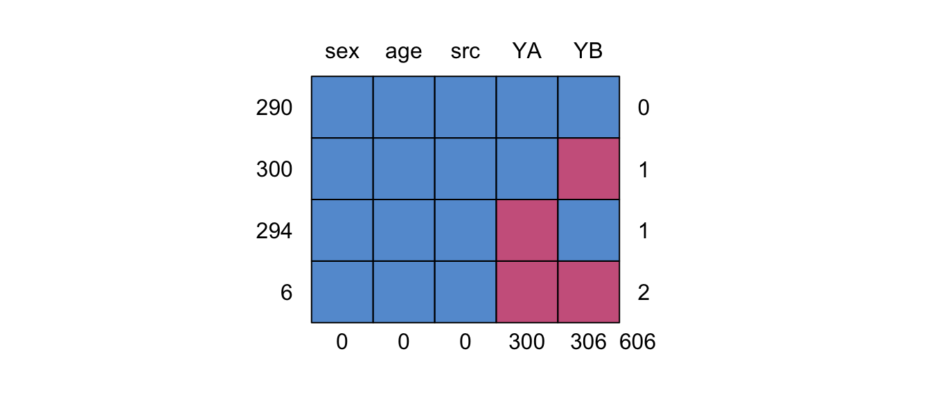
Figure 9.9: Missing data pattern for walking data with a bridge study.

The combined data are available in mice as the dataset walking. Figure 9.9 shows the missing data pattern of the combined data. Observe that YA and YB are now connected by 290 records from the bridge study on sample E. We assume that the data are missing at random. More specifically, the conditional distributions of \(Y_\mathrm{A}\) and \(Y_\mathrm{B}\) given the other item is equivalent across the three sources. Let \(S\) be an administrative variable taking on values \(A\), \(B\) and \(E\) for the three sources. The assumptions are

\[\begin{align} P(Y_\mathrm{A}|Y_\mathrm{B}, X, S=B) & = P(Y_\mathrm{A}|Y_\mathrm{B}, X, S=E)\\ P(Y_\mathrm{B}|Y_\mathrm{A}, X, S=A) & = P(Y_\mathrm{B}|Y_\mathrm{A}, X, S=E) \end{align}\]

where \(X\) contains any relevant covariates, like age and sex, and/or interaction terms. In other words, the way in which \(Y_\mathrm{A}\) depends on \(Y_\mathrm{B}\) and \(X\) is the same in sources \(B\) and \(E\). Likewise, the way in which \(Y_\mathrm{B}\) depends on \(Y_\mathrm{A}\) and \(X\) is the same in sources \(A\) and \(E\). The inclusion of such covariates allows for various forms of differential item functioning (Holland and Wainer 1993).

The two assumptions need critical evaluation. For example, if the respondents in source \(S=E\) answered the items in a different language than the respondents in sources \(A\) or \(B\), then the assumption may not be sensible unless one has great faith in the translation. It is perhaps better then to search for a bridge study that is more comparable. Note that it is only required that the conditional distributions are identical. The imputations remain valid when the samples have different marginal distributions. For efficiency reasons and stability, it is generally advisable to have match samples with similar distribution, but it is not a requirement. The design is known as the common-item nonequivalent groups design (Kolen and Brennan 1995) or the non-equivalent group anchor test (NEAT) design (Dorans 2007).

Multiple imputation on the dataset walking is straightforward.

tau <- NULL
pred <- make.predictorMatrix(walking)
pred[, c("src", "age", "sex")] <- 0
imp <- mice(walking, maxit = 0, m = 10, pred = pred,
            seed = 92786, print = FALSE)
micemill(20)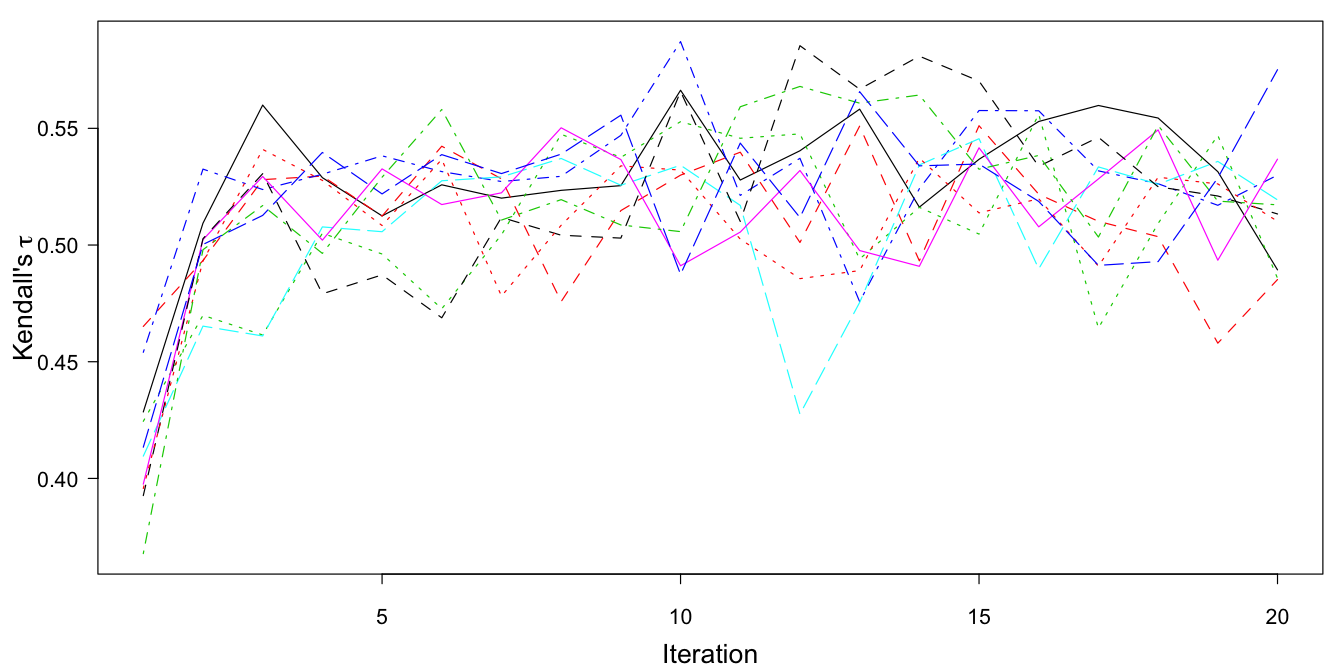

Figure 9.10: The trace plot of Kendall’s \(\tau\) for \(Y_\mathrm{A}\) and \(Y_\mathrm{B}\) using \(m=10\) multiple imputations and 20 iterations. The data are linked by the bridge study.

The behavior of the trace plot is very different now (cf. Figure 9.10). After the first few iterations, the trace lines consistently move around a value of approximately 0.53, with a fairly small range. Thus, after five iterations, the conditional distributions defined by sample E have percolated into the imputations for item A (in sample B) and item B (in sample A).

The behavior of the samplers is dependent on the relative size of the bridge study. In these data, the bridge study is about one third of the total data. If the bridge study is small relative to the other two data sources, the sampler may be slow to converge. As a rule of the thumb, the bridge study should be at least 10% of the total sample size. Also, carefully monitor convergence of the most critical linkages using association measures.

Note that we can also monitor the behavior of \(\hat\theta_\mathrm{AB}\) and \(\hat\theta_\mathrm{BA}\). In order to calculate \(\hat\theta_\mathrm{AB}\) after each iteration we add two statements to the micemill() function:

props <- with(imp, mean(YB[src == "A"] == '0'))
thetaAB <<- rbind(thetaAB, ra(props, simplify = TRUE))

The results are assembled in the variable thetaAB in the working directory. This variable should be initialized as thetaAB <- NULL before milling.

It is possible that the relation between \(Y_\mathrm{A}\) and \(Y_\mathrm{B}\) depends on covariates, like age and sex. If so, including covariates into the imputation model allows for differential item functioning across the covariates. It is perfectly possible to change the imputation model between iterations. For example, after the first 20 iterations (where we impute \(Y_\mathrm{A}\) from \(Y_\mathrm{B}\) and vice versa) we add age and sex as covariates, and do another 20 iterations. This goes as follows:

tau <- NULL
thetaAB <- NULL
pred2 <- pred1 <- make.predictorMatrix(walking)
pred1[, c("src", "age", "sex")] <- 0
pred2[, "src"] <- 0
imp <- mice(walking, maxit = 0, m = 10, pred = pred1,
            seed = 99786)
micemill(20)
imp <- mice(walking, maxit = 0, m = 10, pred = pred2)
micemill(20)

9.4.6 Interpretation

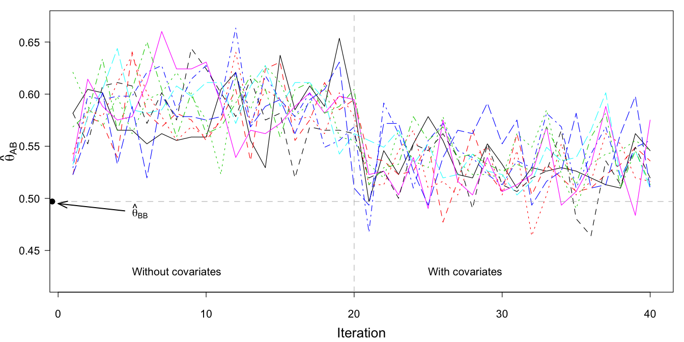
Figure 9.11: Trace plot of \(\hat\theta_\mathrm{AB}\) (proportion of sample A that scores in category 0 of item B) after multiple imputation (\(m=10\)), without covariates (iteration 1–20), and with covariates age and sex as part of the imputation model (iterations 21–40).

Figure 9.11 plots the traces of MICE algorithm, where we calculated \(\theta_\mathrm{AB}\), the proportion of sample A in category 0 of item B. Without covariates, the proportion is approximately 0.587. Under equating, this proportion was found to be equal to 0.807 (cf.Section 9.4.2). The difference between the old (0.807) and the new (0.587) estimate is dramatic. After adding age and sex to the imputation model, \(\theta_\mathrm{AB}\) drops further to about 0.534, close to \(\theta_\mathrm{BB}\), the estimate for population B (0.497).

Table 9.9: Disability and health estimates for populations A and B under four assumptions. \(\hat\theta_\mathrm{AA}\) and \(\hat\theta_\mathrm{BA}\) are the item means on item A for samples A and B, respectively. \(\hat\theta_\mathrm{AB}\) and \(\hat\theta_\mathrm{BB}\) are the proportions of cases into category 0 of item B for samples A and B, respectively. MI-multiple imputation.

Assumption	\(\hat\theta_\mathrm{AA}\)	\(\hat\theta_\mathrm{BA}\)	\(\hat\theta_\mathrm{AB}\)	\(\hat\theta_\mathrm{BB}\)
Simple equating	0.243	0.658	0.807	0.497
Independence	0.243	0.253	0.500	0.497
MI (no covariate)	0.243	0.450	0.587	0.497
MI (covariate)	0.243	0.451	0.534	0.497

Table 9.9 summarizes the estimates from the four analyses. Large differences are found between population A and B when we simply assume that the four categories of both items are identical (simple equating). In this case, population A appears much healthier by both measures. In constrast, if we assume independence between \(Y_\mathrm{A}\) and \(Y_\mathrm{B}\), all differences vanish, so now it appears that the populations A and B are equally healthy. The solutions based on multiple imputation strike a balance between these extremes. Population A is considerably healthier than B on the item mean statistic (0.243 versus 0.451). However, the difference is much smaller on the proportion in category 0, especially after taking age and sex into account. The solutions based on multiple imputation are preferable over the first two because they have taken the relation between items A and B into account.

Which of the four estimates is best? The method of choice is multiple imputation including the covariates. This method not only accounts for the relation between \(Y_A\) and \(Y_B\), but also incorporates the effects of age and sex. Consequently, the method provides estimates with the lowest bias in \(\theta_\mathrm{AB}\) and \(\theta_\mathrm{BA}\).

9.4.7 Conclusion

Incomparability of data is a key problem in many fields. It is natural for scientists to adapt, refine and tweak measurement procedures in the hope of obtaining better data. Frequent changes, however, will hamper comparisons.

Equating categories is widely practiced to “make the data comparable.” It is often not realized that recoding and equating data amplify differences. The degree of exaggeration is inversely related to Kendall’s \(\tau\). For the item mean statistic, the difference in mean walking disability after equating is about twice the size of that under multiple imputation. Also, the estimate of 0.807 after simple equating is a gross overestimate. Overstated differences between populations may spur inappropriate interventions, sometimes with substantial financial consequences. Unless backed up by appropriate data, equating categories is not a solution.

The section used multiple imputation as a natural and attractive alternative. The first major application of multiple imputation addressed issues of comparability (Clogg et al. 1991). The advantage is that bureau A can interpret the information of bureau B using the scale of bureau A, and vice versa. The method provides possible contingency tables of items A and B that could have been observed if both had been measured. Dorans (2007) describes techniques for creating valid equating tables. Such tables convert the score of instrument A into that of instrument B, and vice versa. The requirements for constructing such tables are extremely high: the measured constructs should be equal, the reliability should be equal, the conversion of B to A should be the inverse of that from B to A (symmetry), it should not matter whether A or B is measured and the table should be independent of the population. Holland (2007) presents a logical sequence of linking methods that progressively moves toward higher forms of equating. Multiple imputation in general fails on the symmetry requirement, as it produces \(m\) scores on B for one score of A, and thus cannot be invertible. The method as presented here can be seen as a first step toward obtaining formal equating of test items. It can be improved by correcting for the reliabilities of both items. This is an area of future research.

For simplicity, the statistical analyses used only one bridge item. In general, better strategies are possible. It is wise to include as many bridge items as there are. Also, linking and equating at the sub-scale and scale levels could be done (Dorans 2007). The double-coded data could also comprise a series of vignettes (Salomon, Tandon, and Murray 2004). The use of such strategies in combination with multiple imputation has yet to be explored.