10.1 Correcting for selective drop-out
Panel attrition is a problem that plagues all studies in which the same people are followed over time. People who leave the study are called drop-outs. The persons who drop out may be systematically different from those who remain, thus providing an opportunity for bias. This section assumes that the drop-out mechanism is MAR and that the parameters of the complete-data model and the response mechanism are distinct (cf. Section 2.2.5). Techniques for nonignorable drop-outs are described by Little (1995), Diggle et al. (2002), Daniels and Hogan (2008) and Wu (2010).
10.1.1 POPS study: 19 years follow-up
The Project on Preterm and Small for Gestational Age Infants (POPS) is an ongoing collaborative study in the Netherlands on the long-term effect of prematurity and dysmaturity on medical, psychological and social outcomes. The cohort was started in 1983 and enrolled 1338 infants with a gestational age below 32 weeks or with a birth weight of below 1500 grams (Verloove-Vanhorick et al. 1986). Of this cohort, 312 infants died in the first 28 days, and another 67 children died between the ages of 28 days and 19 years, leaving 959 survivors at the age of 19 years. Intermediate outcome measures from earlier follow-ups were available for 89% of the survivors at age 14 (\(n\) = 854), 77% at age 10 (\(n\) = 712), 84% at age 9(\(n\) = 813), 96% at age 5 (\(n\) = 927) and 97% at age 2 (\(n\) = 946).
To study the effect of drop-out, Hille et al. (2005) divided the 959 survivors into three response groups:
Full responders were examined at an outpatient clinic and completed the questionnaires (\(n\) = 596);
Postal responders only completed the mailed questionnaires (\(n\) = 109);
Nonresponders did not respond to any of the mailed requests or telephone calls, or could not be traced (\(n\) = 254).
10.1.2 Characterization of the drop-out
Of the 254 nonresponders, 38 children (15%) did not comply because they were “physically or mentally unable to participate in the assessment.” About half of the children (132, 52%) refused to participate. No reason for drop-out was known for 84 children (33%).
| Variable | All | Full responders | Postal responders | Non-responders | ||||
|---|---|---|---|---|---|---|---|---|
| \(n\) | 959 | 596 | 109 | 254 | ||||
| Sex | ||||||||
| Boy | 497 | (51.8) | 269 | (45.1) | 60 | (55.0) | 168 | (66.1) |
| Girl | 462 | (48.2) | 327 | (54.9) | 49 | (45.0) | 86 | (33.9) |
| Origin | ||||||||
| Dutch | 812 | (84.7) | 524 | (87.9) | 96 | (88.1) | 192 | (75.6) |
| Non-Dutch | 147 | (15.3) | 72 | (12.1) | 13 | (11.9) | 62 | (24.4) |
| Maternal education | ||||||||
| Low | 437 | (49.9) | 247 | (43.0) | 55 | (52.9) | 135 | (68.2) |
| Medium | 299 | (34.1) | 221 | (38.5) | 31 | (29.8) | 47 | (23.7) |
| High | 140 | (16.0) | 106 | (18.5) | 18 | (17.3) | 16 | (8.1) |
| SES | ||||||||
| Low | 398 | (42.2) | 210 | (35.5) | 48 | (44.4) | 140 | (58.8) |
| Medium | 290 | (30.9) | 193 | (32.6) | 31 | (28.7) | 66 | (27.7) |
| High | 250 | (26.7) | 189 | (31.9) | 29 | (26.9) | 32 | (13.4) |
| Handicap at age 14 | ||||||||
| Normal | 480 | (50.8) | 308 | (51.7) | 42 | (38.5) | 130 | (54.2) |
| Impairment | 247 | (26.1) | 166 | (27.9) | 36 | (33.0) | 45 | (18.8) |
| Mild | 153 | (16.2) | 101 | (16.9) | 16 | (14.7) | 36 | (15.0) |
| Severe | 65 | (6.9) | 21 | (3.5) | 15 | (13.8) | 29 | (12.1) |
Table 10.1 lists some of the major differences between the three response groups. Compared to the postal and nonresponders, the full response group consists of more girls, contains more Dutch children, has higher educational and social economic levels and has fewer handicaps. Clearly, the responders form a highly selective subgroup in the total cohort.
Differential drop-out from the less healthy children leads to an obvious underestimate of disease prevalence. For example, the incidence of handicaps would be severely underestimated if based on data from the full responders only. In addition, selective drop-out could bias regression parameters in predictive models if the reason for drop-out is related to the outcome of interest. This may happen, for example, if we try to predict handicaps at the age of 19 years from the full responders only. Thus, statistical parameters may be difficult to interpret in the presence of selective drop-out.
10.1.3 Imputation model
The primary interest of the investigators focused on 14 different outcomes at 19 years: cognition, hearing, vision, neuromotor functioning, ADHD, respiratory symptoms, height, BMI, health status (Health Utilities Index Mark 3), perceived health (London Handicap Scale), coping, self-efficacy, educational attainment and occupational activities. Since it is inefficient to create a multiply imputed dataset for each outcome separately, the goal is to construct one set of imputed data that is used for all analyses.
For each outcome, the investigator created a list of potentially relevant predictors according to the predictor selection strategy set forth in Section 6.3.2. In total, this resulted in a set of 85 unique variables. Only four of these were completely observed for all 959 children. Moreover, the information provided by the investigators was coded (in Microsoft Excel) as an 85 \(\times\) 85 predictor matrix that is used to define the imputation model.
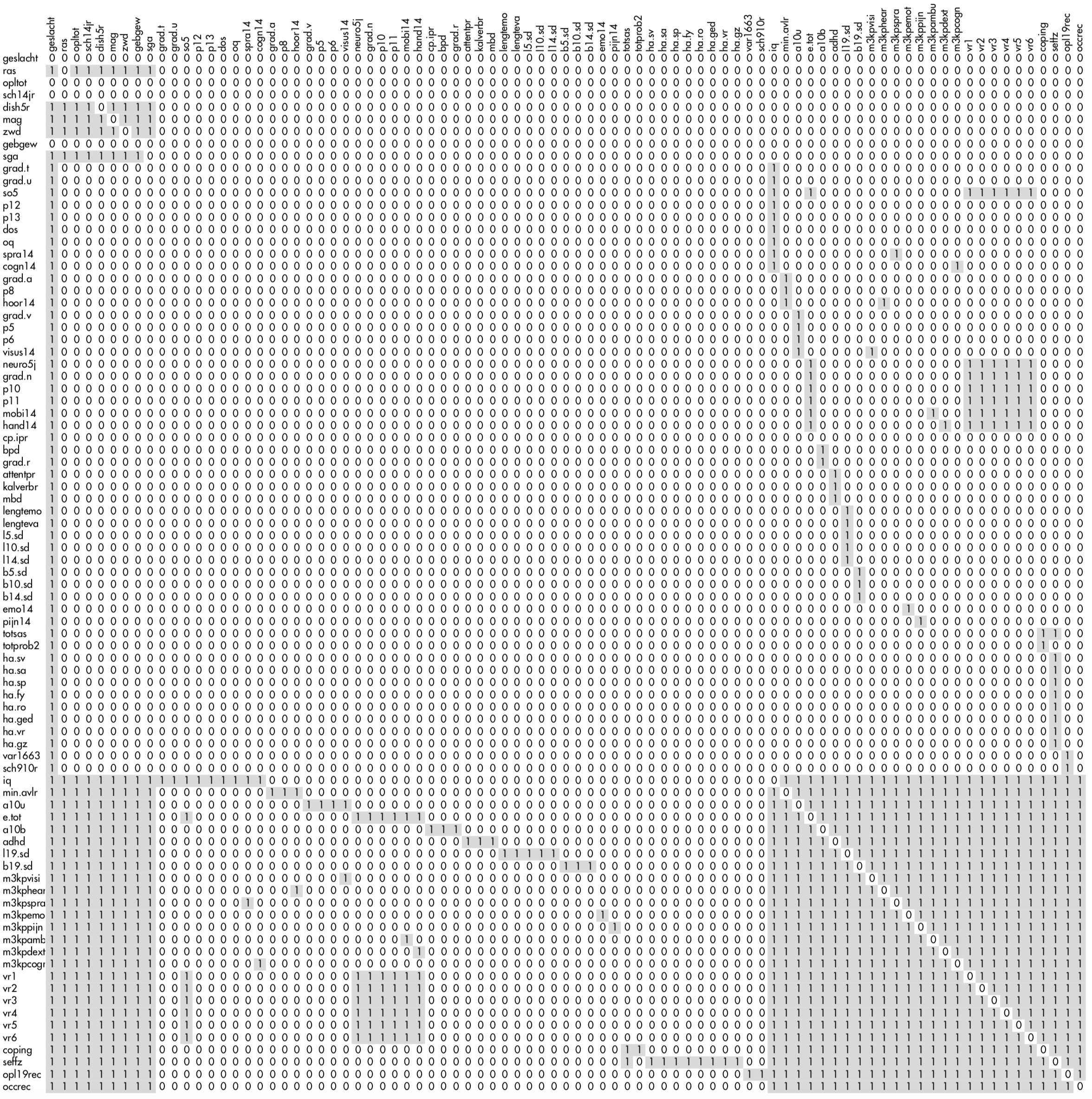
Figure 10.1: The 85 \(\times\) 85 predictor matrix used in the POPS study. The gray parts signal the column variables that are used to impute the row variable.
Figure 10.1 shows a miniature version of the predictor matrix. The dark cell indicates that the column variable is used to impute the row variable. Note the four complete variables with rows containing only zeroes. There are three blocks of variables. The first nine variables (Set 1: geslacht-sga) are potential confounders that should be controlled for in all analyses. The second set of variables (Set 2: grad.t-sch910r) are variables measured at intermediate time points that appear in specific models. The third set of variables (Set 3: iq-occrec) are the incomplete outcomes of primary interest collected at the age of 19 years. The imputation model is defined such that:
All variables in Set 1 are used as predictors to impute Set 1, to preserve relations between them;
All variables in Set 1 are used as predictors to impute Set 3, because all variables in Set 1 appear in the complete-data models of Set 3;
All variables in Set 3 are used as predictors to impute Set 3, to preserve the relation between the variables measured at age 19;
Selected variables in Set 2 that appear in complete-data models are used as predictors to impute specific variables in Set 3;
Selected variables in Set 3 are “mirrored” to impute incomplete variables in Set 2, so as to maintain consistency between Set 2 and Set 3 variables;
The variable
geslacht(sex) is included in all imputation models.
This setup of the predictor matrix avoids fitting unwieldy imputation models, while maintaining the relations of scientific interest.
10.1.4 A solution “that does not look good”
The actual imputations can be produced by
imp1 <- mice(data, pred = pred, maxit = 20,
             seed = 51121, print = FALSE)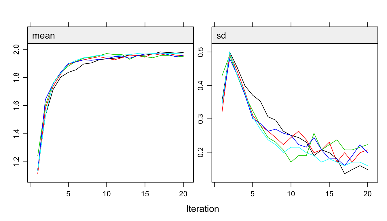
Figure 10.2: Trace lines of the MICE algorithm for the variable a10u illustrating problematic convergence.
The number of iterations is set to 20 because the trace lines from the MICE algorithm show strong initial trends and slow mixing.
Figure 10.2 plots the trace lines of the binary variable a10u, an indicator of visual disabilities. The behavior of these trace lines looks suspect, especially for a10u. The mean of a10u (left side) of the imputed values converges to a value near 1.9, while the standard deviation (right side) drops below that variability that is found in the data. Since the categories are coded as 1 = no problem and 2 = problem, a value of 1.9 actually implies that 90% of the nonresponders would have a problem. The observed prevalence of a10u in the full responders is only 1.5%, so 90% is clearly beyond any reasonable value.
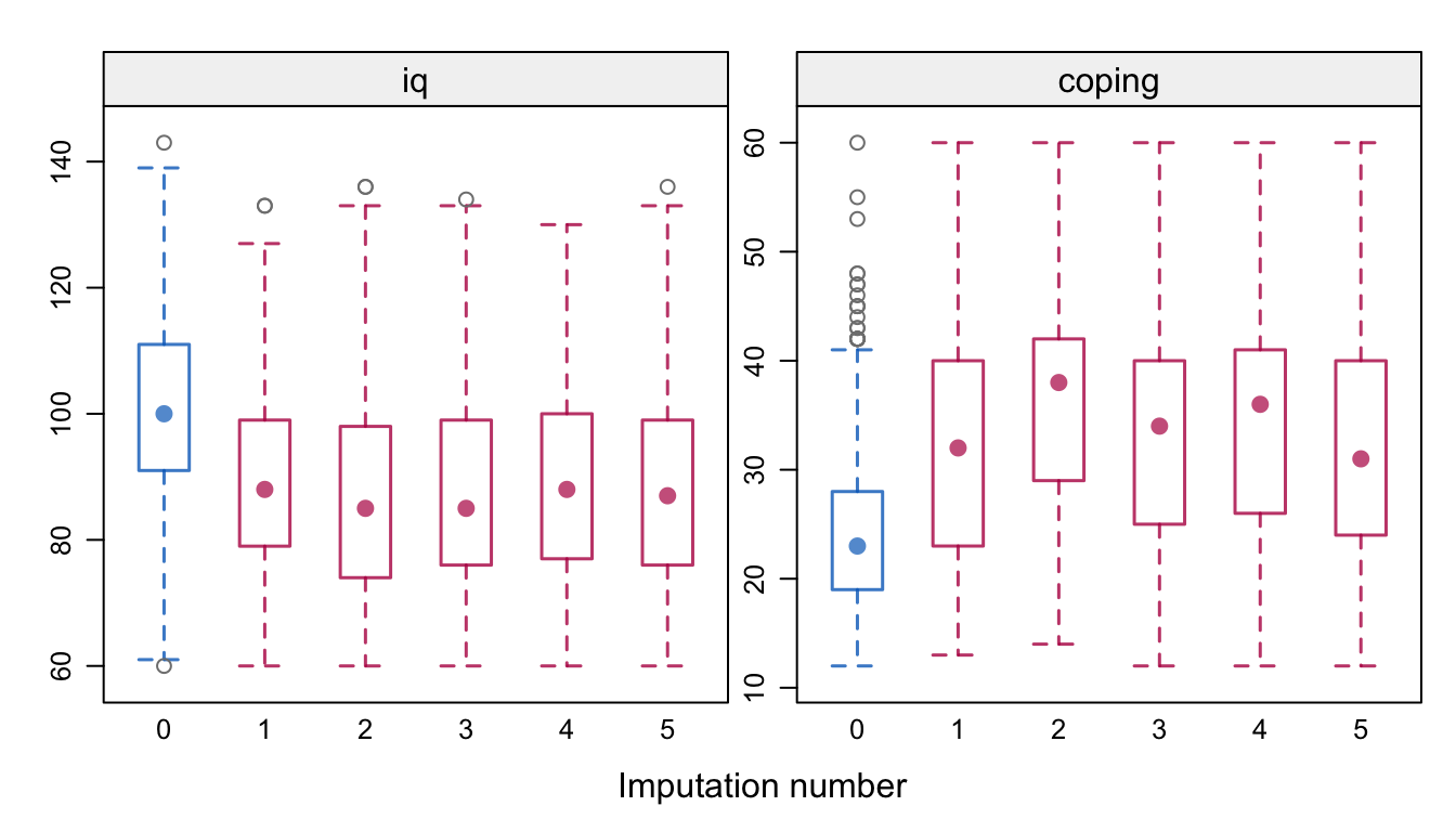
Figure 10.3: Distributions (observed and imputed) of IQ and coping score at 19 years in the POPS study for the imputation model in Figure 10.1.
In addition, iq and coping move into remote territories. Figure 10.3 illustrates that the imputed values for iq appear unreasonably low, whereas for coping they appear unreasonably high. What is happening here?
The phenomenon we see illustrates a weakness (or feature) of the MICE algorithm that manifests itself when the imputation model is overparametrized relative to the available information. The source of the problem lies in the imputation of the variables in Set 3, the measurements at 19 years. We specified that all variables in Set 3 should impute each other, with the idea of preserving the multivariate relations between these variables. For 254 out of 959 children (26.5%), we do not have any information at age 19. The MICE algorithm starts out by borrowing information from the group of responders, and then quickly finds out that it can create imputations that are highly correlated. However, the imputed values do not look at all like the observed data, and are more like multivariate outliers that live in an extreme part of the data space.
There are several ways to alleviate the problem. The easiest approach is to remove the 254 nonresponders from the data. This is a sensible approach if the analysis focuses on determinants of 19-year outcomes, but it is not suitable for making inferences on the marginal outcome distribution of the entire cohort. A second approach is to simplify the model. Many of the 19-year outcomes are categorical, and we reduce the number of parameters drastically by applying predictive mean matching to these outcomes. A third approach would be to impute all outcomes as a block. This would find potential donors among the observed data, and impute all outcomes simultaneously. This removes the risk of artificially inflating the relations among outcomes, and is a promising alternative. Finally, the approach we follow here is to simplify the imputation model by removing the gray block in the lower-right part of Figure 10.1. The relation between the outcomes would then only be maintained through their relation with predictors measured at other time points. It is easy to change and rerun the model as:
pred[61:86, 61:86] <- 0
imp2 <- mice(data, pred = pred, maxit = 20,
             seed = 51121, print = FALSE)
These statements produce imputations with marginal distributions much closer to the observed data. Also, the trace lines now show normal behavior (not shown). Convergence occurs rapidly in about 5-10 iterations.
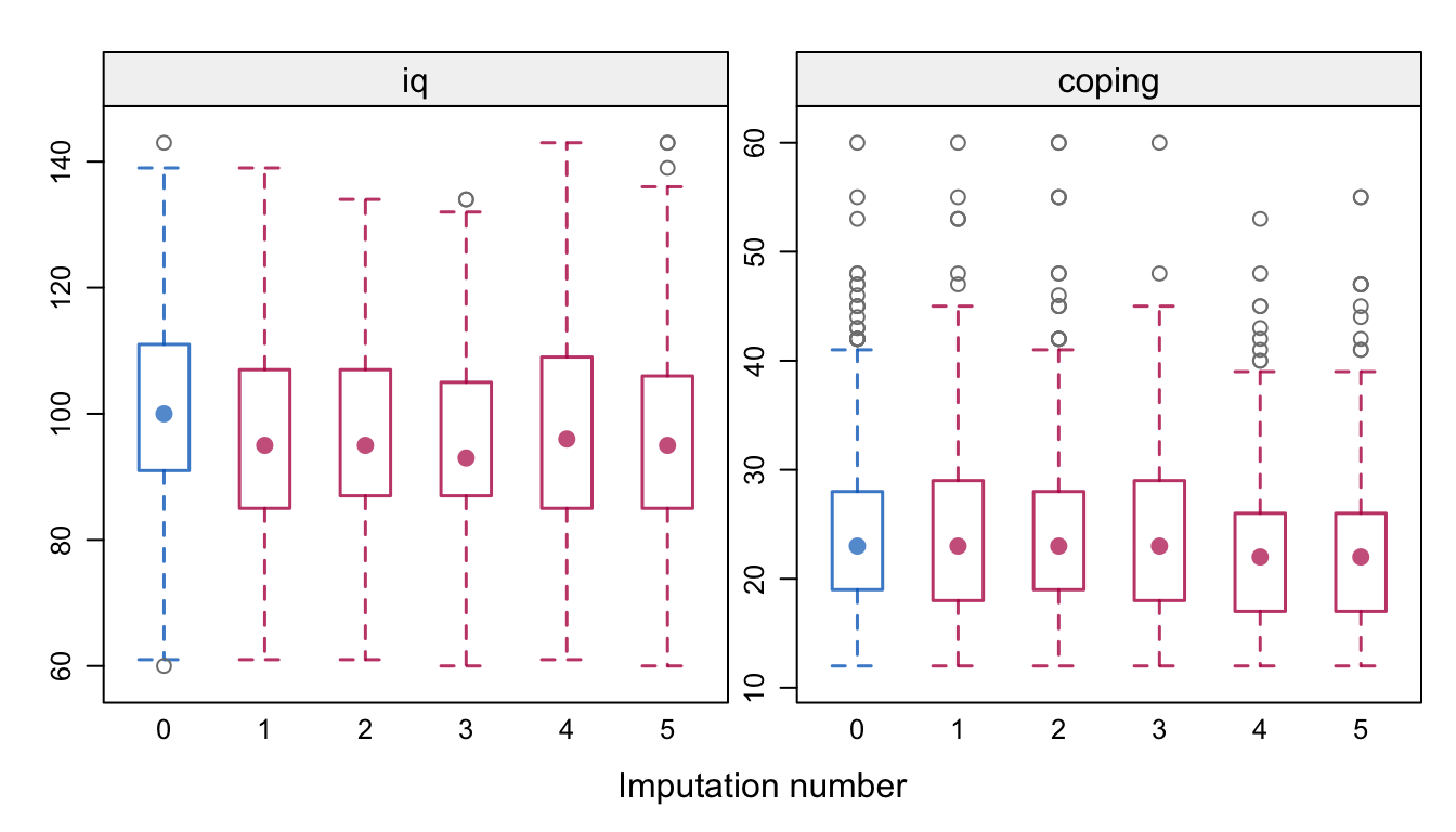
Figure 10.4: Distributions (observed and imputed) of IQ and coping score at 19 years in the POPS study for the simplified imputation model.
Figure 10.4 displays the distributions of IQ and coping. The nonrespondents have slightly lower IQ scores, but not as extreme as in Figure 10.3. There are now hardly any differences in coping.
10.1.5 Results
Table 10.2 provides estimates of the percentage of three health problems, both uncorrected and corrected for selective drop-out. As expected, all estimates are adjusted upward. Note that the prevalence of visual problems tripled to 4.7% after correction. While this increase is substantial, it is well within the range of odds ratios of 2.6 and 4.4 reported by Hille et al. (2005). The adjustment shows that prevalence estimates in the whole group can be substantially higher than in the group of full responders. Hille et al. (2007) provide additional and more detailed results.
| \(n_{\rm obs}\) | Full | \(n\) | All | |||
|---|---|---|---|---|---|---|
| Severe visual handicap | 690 | 1.4 | (0.5-2.3) | 959 | 4.7 | (1.0-10.9) |
| Asthma, bronchitis, CARA | 690 | 8.0 | (5.9-10.0) | 959 | 9.2 | (6.9-11.2) |
| ADHD | 666 | 4.7 | (3.1-6.3) | 959 | 5.7 | (3.8-10.8) |
10.1.6 Conclusion
Many studies are plagued by selective drop-out. Multiple imputation provides an intuitive way to adjust for drop-out, thus enabling estimation of statistics relative to the entire cohort rather than the subgroup. The method assumes MAR. The formulation of the imputation model requires some care. Section 10.1.3 outlines a simple strategy to specify the predictor matrix to fit an imputation model for multiple uses. This methodology is easily adapted to other studies.
Section 10.1.4 illustrates that multiple imputation is not without dangers. The imputations produced by the initial model were far off, which underlines the importance of diagnostic evaluation of the imputed data. A disadvantage of the approach taken to alleviate the problem is that it preserves the relations between the variables in Set 3 only insofar as they are related through their common predictors. These relations may thus be attenuated. Some alternatives were highlighted, and an especially promising one is to impute blocks of variables (cf. Section 4.7.2). Whatever is done, it is important to diagnose aberrant algorithmic behavior, and decide on an appropriate strategy to prevent it given the scientific questions at hand.