3.1 How to generate multiple imputations

This section illustrates five ways to create imputations for a single incomplete continuous target variable. We use dataset number 88 in Hand et al. (1994), which is also part of the MASS library under the name whiteside. Mr. Whiteside of the UK Building Research Station recorded the weekly gas consumption (in 1000 cubic feet) and average external temperature (in \(^\circ\mathrm{C}\)) at his own house in south-east England for two heating seasons (1960 and 1961). The house thermostat was set at 20\(^\circ\mathrm{C}\) throughout.

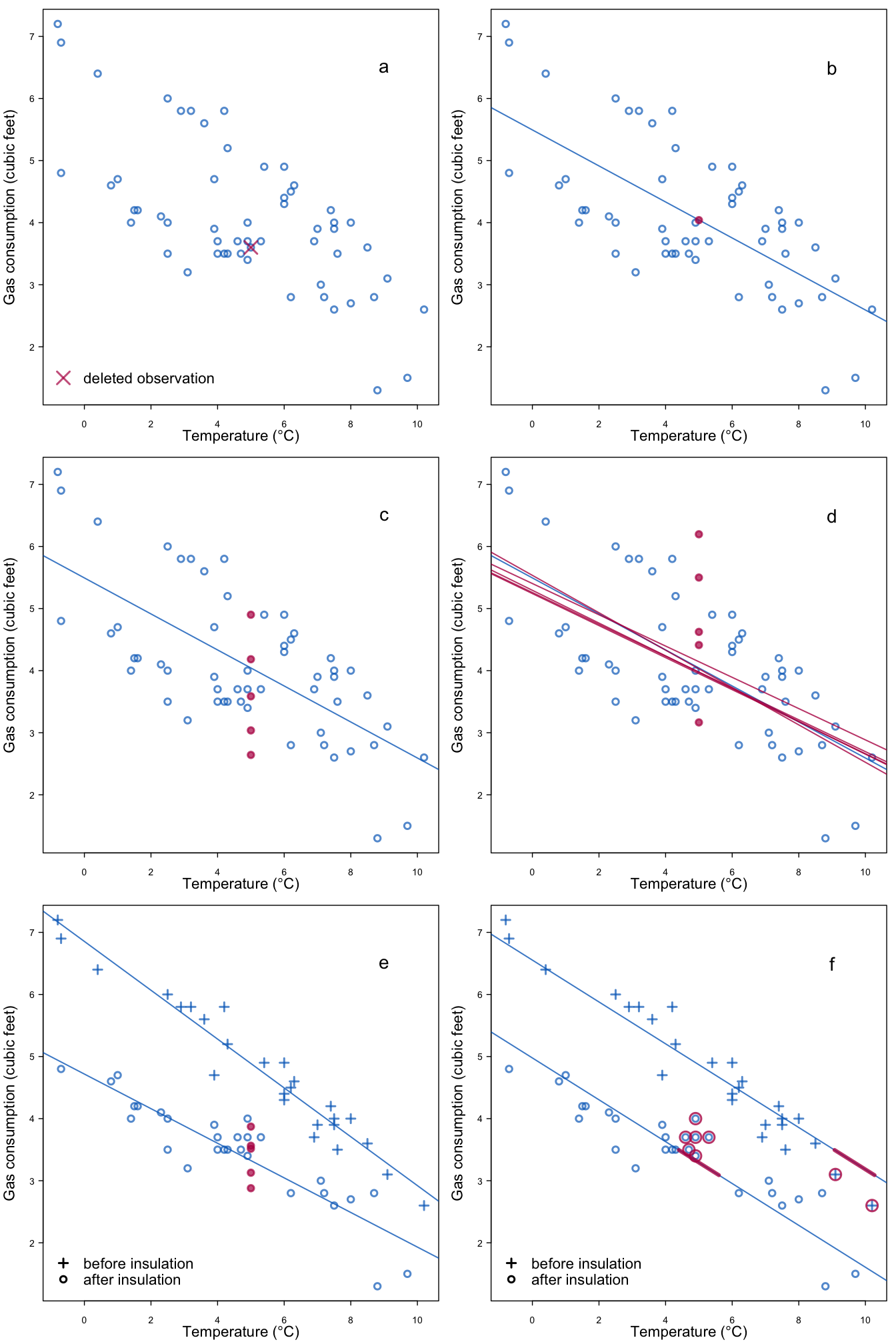
Figure 3.1: Five ways to impute missing gas consumption for a temperature of 5\(^\circ\mathrm{C}\): (a) no imputation; (b) predict; (c) predict + noise; (d) predict + noise + parameter uncertainty; (e) two predictors; (f) drawing from observed data.

Figure 3.1a plots the observed data. More gas is needed in colder weeks, so there is an obvious relation in the data. The dataset is complete, but for the sake of argument suppose that the gas consumption in row 47 of the data is missing. The temperature at this deleted observation is equal to 5\(^\circ\mathrm{C}\). How would we create multiple imputations for the missing gas consumption?

3.1.1 Predict method

A first possibility is to calculate the regression line, and take the imputation from the regression line. The estimated regression line is equal to \(y=5.49 - 0.29 x\), so the value at \(x=5\) is \(5.49-0.29 \times 5 = 4.04\). Figure 3.1b shows where the imputed value is. This is actually the “best” value in the sense that it is the most likely one under the regression model. However, even the best value may differ from the actual (unknown) value. In fact, we are uncertain about the true gas consumption. Predicted values, however, do not portray this uncertainty, and therefore cannot be used as multiple imputations.

3.1.2 Predict + noise method

We can improve upon the prediction method by adding an appropriate amount of random noise to the predicted value. Let us assume that the observed data are normally distributed around the regression line. The estimated standard deviation in the Whiteside data is equal to 0.86 cubic feet. The idea is now to draw a random value from a normal distribution with a mean of zero and a standard deviation of 0.86, and add this value to the predicted value. The underlying assumption is that the distribution of gas consumption of the incomplete observation is identical to that in the complete cases.

We can repeat the draws to get multiple synthetic values around the regression line. Figure 3.1c illustrates five such drawn values. On average, the synthetic values will be equal to the predicted value. The variability in the values reflects that fact that we cannot accurately predict gas consumption from temperature.

3.1.3 Predict + noise + parameter uncertainty

Adding noise is a major step forward, but not quite right. The method in the previous section requires that the intercept, the slope and the standard deviation of the residuals are known. However, the values of these parameters are typically unknown, and hence must be estimated from the data. If we had drawn a different sample from the same population, then our estimates for the intercept, slope and standard deviation would be different, perhaps slightly. The amount of extra variability is strongly related to the sample size, with smaller samples yielding more variable estimates.

The parameter uncertainty also needs to be included in the imputations. There are two main methods for doing so. Bayesian methods draw the parameters directly from their posterior distributions, whereas bootstrap methods resample the observed data and re-estimate the parameters from the resampled data.

Figure 3.1d shows five sampled regression lines calculated by Bayesian sampling. Imputed values are now defined as the predicted value of the sampled line added with noise, as in Section 3.1.2.

3.1.4 A second predictor

The dataset actually contains a second predictor that indicates whether the house was insulated or not. Incorporating this extra information reduces the uncertainty of the imputed values.

Figure 3.1e shows the same data, but now flagged according to insulation status. Two regression lines are shown, one for the insulated houses and the other for the non-insulated houses. It is clear that less gas is needed after insulation. Suppose we know that the external temperature is 5\(^\circ\mathrm{C}\) and that the house was insulated. How do we create multiple imputation given these two predictors?

We apply the same method as in Section 3.1.3, but now using the regression line for the insulated houses. Figure 3.1e shows the five values drawn for this method. As expected, the distribution of the imputed gas consumption has shifted downward. Moreover, its variability is lower, reflecting that fact that gas consumption can be predicted more accurately as insulation status is also known.

3.1.5 Drawing from the observed data

Figure 3.1f illustrates an alternative method to create imputations. As before, we calculate the predicted value at 5\(^\circ\mathrm{C}\) for an insulated house, but now select a small number of candidate donors from the observed data. The selection is done such that the predicted values are close. We then randomly select one donor from the candidates, and use the observed gas consumption that belongs to that donor as the synthetic value. The figure illustrates the candidate donors, not the imputations.

This method is known as predictive mean matching, and always finds values that have been actually observed in the data. The underlying assumption is that within the group of candidate donors gas consumption has the same distribution in donors and receivers. The variability between the imputations over repeated draws is again a reflection of the uncertainty of the actual value.

3.1.6 Conclusion

In summary, prediction methods are not suitable to create multiple imputations. Both the inherent prediction error and the parameter uncertainty should be incorporated into the imputations. Adding a relevant extra predictor reduces the amount of uncertainty, and leads to more efficient estimates later on. The text also highlights an alternative that draws imputations from the observed data. The imputation methods discussed in this chapter are all variations on this basic idea.