1.1 The problem of missing data
1.1.1 Current practice
The mean of the numbers 1, 2 and 4 can be calculated in R as
y <- c(1, 2, 4)
mean(y)
[1] 2.33where y is a vector containing three numbers, and where mean(y) is the R expression that returns their mean. Now suppose that the last number is missing. R indicates this by the symbol NA, which stands for “not available”:
y <- c(1, 2, NA)
mean(y)
[1] NAThe mean is now undefined, and R informs us about this outcome by setting the mean to NA. It is possible to add an extra argument na.rm = TRUE to the function call. This removes any missing data before calculating the mean:
mean(y, na.rm = TRUE)[1] 1.5This makes it possible to calculate a result, but of course the set of observations on which the calculations are based has changed. This may cause problems in statistical inference and interpretation.
It gets worse with multivariate analysis. For example, let us try to predict daily ozone concentration (ppb) from wind speed (mph) using the built-in airquality dataset. We fit a linear regression model by calling the lm() function to predict daily ozone levels, as follows:
fit <- lm(Ozone ~ Wind, data = airquality)
# Error in na.fail.default: missing values in object}
Many R users have seen this message. The code cannot continue because there are missing values. One way to circumvent the problem is to omit any incomplete records by specifying the na.action = na.omit argument to lm(). The regression weights can now be obtained as
fit <- lm(Ozone ~ Wind, data = airquality, na.action = na.omit)This works. For example, we may produce diagnostic plots by plot(fit) to study the quality of the model. In practice, it is cumbersome to supply the na.action() function each time. We can change the setting in options as
options(na.action = na.omit)which eliminates the error message once and for all. Users of other software packages like SPSS, SAS and Stata enjoy the “luxury” that this deletion option has already been set for them, so the calculations can progress silently. Next, we wish to plot the predicted ozone levels against the observed data, so we use predict() to calculate the predicted values, and add these to the data to prepare for plotting.
airquality2 <- cbind(airquality, predict(fit))
# Error: arguments imply differing number of rows: 153, 116
Argg… that doesn’t work either. The error message tells us that the two datasets have a different number of rows. The airquality data has 153 rows, whereas there are only 116 predicted values. The problem, of course, is that there are missing data. The lm() function dropped any incomplete rows in the data. We find the indices of the first six cases by
head(na.action(fit)) 5 10 25 26 27 32
5 10 25 26 27 32 The total number of deleted cases is found as
naprint(na.action(fit))[1] "37 observations deleted due to missingness"The number of missing values per variable in the data is
colSums(is.na(airquality)) Ozone Solar.R Wind Temp Month Day
37 7 0 0 0 0 so in our regression model, all 37 deleted cases have missing ozone scores.
Removing the incomplete cases prior to analysis is known as listwise deletion or complete-case analysis. In R, there are two related functions for the subset of complete cases, na.omit() and complete.cases().
Figure 1.1 plots the predicted against the observed values. Here we adopt the Abayomi convention for the colors (Abayomi, Gelman, and Levy 2008): Blue refers to the observed part of the data, red to the synthetic part of the data (also called the imputed values or imputations), and black to the combined data (also called the imputed data or completed data). The printed version of the first edition of this book used gray instead of blue. The blue points on the left are all from the complete cases, whereas the figure on the right plots the points for the incomplete cases (in red). Since there are no measured ozone levels in that part of the data, the possible values are indicated by 37 horizontal lines.
airquality2 <- cbind(na.omit(airquality[, c("Ozone", "Wind")]),
                     predicted = predict(fit))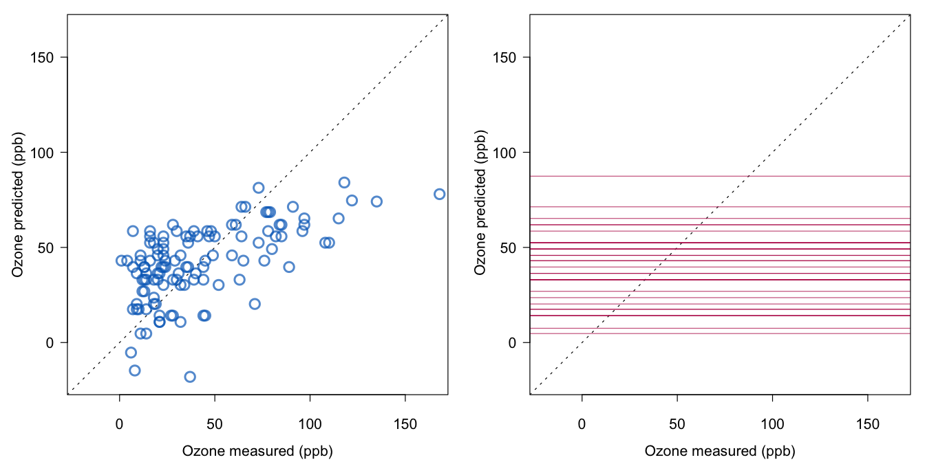
Figure 1.1: Predicted versus measured ozone levels for the observed (left, blue) and missing values (right, red).
Listwise deletion allows the calculations to proceed, but it may introduce additional complexities in interpretation. Let’s try to find a better predictive model by including solar radiation (Solar.R) into the model as
fit2 <- lm(Ozone ~ Wind + Solar.R, data = airquality)
naprint(na.action(fit2))
[1] "42 observations deleted due to missingness"Observe that the number of deleted days increased is now 42 since some rows had no value for Solar.R. Thus, changing the model altered the sample.
There are methodological and statistical issues associated with this procedure. Some questions that come to mind are:
Can we compare the regression coefficients from both models?
Should we attribute differences in the coefficients to changes in the model or to changes in the subsample?
Do the estimated coefficients generalize to the study population?
Do we have enough cases to detect the effect of interest?
Are we making the best use of the costly collected data?
Getting the software to run is one thing, but this alone does not address the challenges posed by the missing data. Unless the analyst, or the software vendor, provides some way to work around the missing values, the analysis cannot continue because calculations on missing values are not possible. There are many approaches to circumvent this problem. Each of these affects the end result in a different way. Some solutions are clearly better than others, and there is no solution that will always work. This chapter reviews the major approaches, and discusses their advantages and limitations.
1.1.2 Changing perspective on missing data
The standard approach to missing data is to delete them. It is illustrative to search for missing values in published data. Hand et al. (1994) published a highly useful collection of small datasets across the statistical literature. The collection covers an impressive variety of topics. Only 13 out of the 510 datasets in the collection actually had a code for the missing data. In many cases, the missing data problem has probably been “solved” in some way, usually without telling us how many missing values there were originally. It is impossible to track down the original data for most datasets in Hand’s book. However, we can easily do this for dataset number 357, a list of scores of 34 athletes in 10 sport events at the 1988 Olympic decathlon in Seoul. The table itself is complete, but a quick search on the Internet revealed that initially 39 instead of 34 athletes participated. Five of them did not finish for various reasons, including the dramatic disqualification of the German favorite Jürgen Hingsen because of three false starts in the 100-meter sprint. It is probably fair to assume that deletion occurred silently in many of the other datasets.
The inclination to delete the missing data is understandable. Apart from the technical difficulties imposed by the missing data, the occurrence of missing data has long been considered a sign of sloppy research. It is all too easy for a referee to write:
This study is weak because of the large amount of missing data.
Publication chances are likely to improve if there is no hint of missingness. Orchard and Woodbury (1972, 697) remarked:
Obviously the best way to treat missing data is not to have them.
Though there is a lot of truth in this statement, Orchard and Woodbury realized the impossibility of attaining this ideal in practice. The prevailing scientific practice is to downplay the missing data. Reviews on reporting practices are available in various fields: clinical trials (Wood, White, and Thompson 2004; Powney et al. 2014; Díaz-Ordaz et al. 2014; Akl et al. 2015), cancer research (Burton and Altman 2004), educational research (Peugh and Enders 2004), epidemiology (Klebanoff and Cole 2008; Karahalios et al. 2012), developmental psychology (Jeliĉić, Phelps, and Lerner 2009), general medicine (Mackinnon 2010), developmental pediatrics (Aylward, Anderson, and Nelson 2010), and otorhinolaryngology, head and neck surgery (Netten et al. 2017). The picture that emerges from these studies is quite consistent:
The presence of missing data is often not explicitly stated in the text;
Default methods, such as listwise deletion are used without mentioning them;
Different tables are based on different sample sizes;
Model-based missing data methods, such as direct likelihood, full information maximum likelihood and multiple imputation, are notably underutilized.
Helpful resources include the STROBE (Vandenbroucke et al. 2007) and CONSORT checklists and flow charts (Schulz, Altman, and Moher 2010). Gomes et al. (2016) showed cases where the subset of full patient-reported outcomes is a selective, leading to misleading results. Palmer et al. (2018) suggested a classification scheme for the reasons of nonresponse in patient-reported outcomes.
Missing data are there, whether we like it or not. In the social sciences, it is nearly inevitable that some respondents will refuse to participate or to answer certain questions. In medical studies, attrition of patients is very common. The theory, methodology and software for handling incomplete data problems have been vastly expanded and refined over the last decades. The major statistical analysis packages now have facilities for performing the appropriate analyses. This book aims to contribute to a better understanding of the issues involved, and provides a methodology for dealing with incomplete data problems in practice.