7.10 Guidelines and advice
Many new multilevel methods have seen the light in the last five years. The comparative work as summarized above spawned a wealth of information. This section provides advice, guidelines and worked examples aimed to assist the applied statistician in solving practical multilevel imputation problems. The field moves rapidly, so the recommendations given here may change as more detailed comparative works become available in the future.
The advice given here builds upon the recommendations and code examples given in Table 6 in Grund, Lüdtke, and Robitzsch (2018b), supplemented by some of my personal biases.
There is not yet a fully satisfactory strategy for handling interactions with FCS. In this section, I will use passive imputation (Van Buuren and Groothuis-Oudshoorn 2000), a technique that allows the user to specify deterministic relations between variables, which, amongst others, is useful for calculating interaction effects within the MICE algorithm. I will use passive imputation to enrich univariate imputation models with two-order interactions, in an attempt to preserve higher-order relations in the data. Passive imputation works reasonably well, and it is easy to apply in standard software, but it is only an approximate solution. In general, the joint distribution of the dependent and explanatory variables tends to become complex when the substantive model contains interactions (Seaman, Bartlett, and White 2012; Kim, Sugar, and Belin 2015).
We revisit the brandsma data use in Chapters 4 and 5 of Snijders and Bosker (2012). For reasons of clarity, the code examples are restricted to a subset of six variables.
data("brandsma", package = "mice")
dat <- brandsma[, c("sch", "pup", "lpo",
                    "iqv", "ses", "ssi")]
There is one cluster variable (sch), one administrative variable (pup), one outcome variable at the pupil level (lpo), two explanatory variables at the pupil level (iqv, ses) and one explanatory variable at the school level (ssi). The cluster variable and pupil number are complete, whereas the others contain missing values.
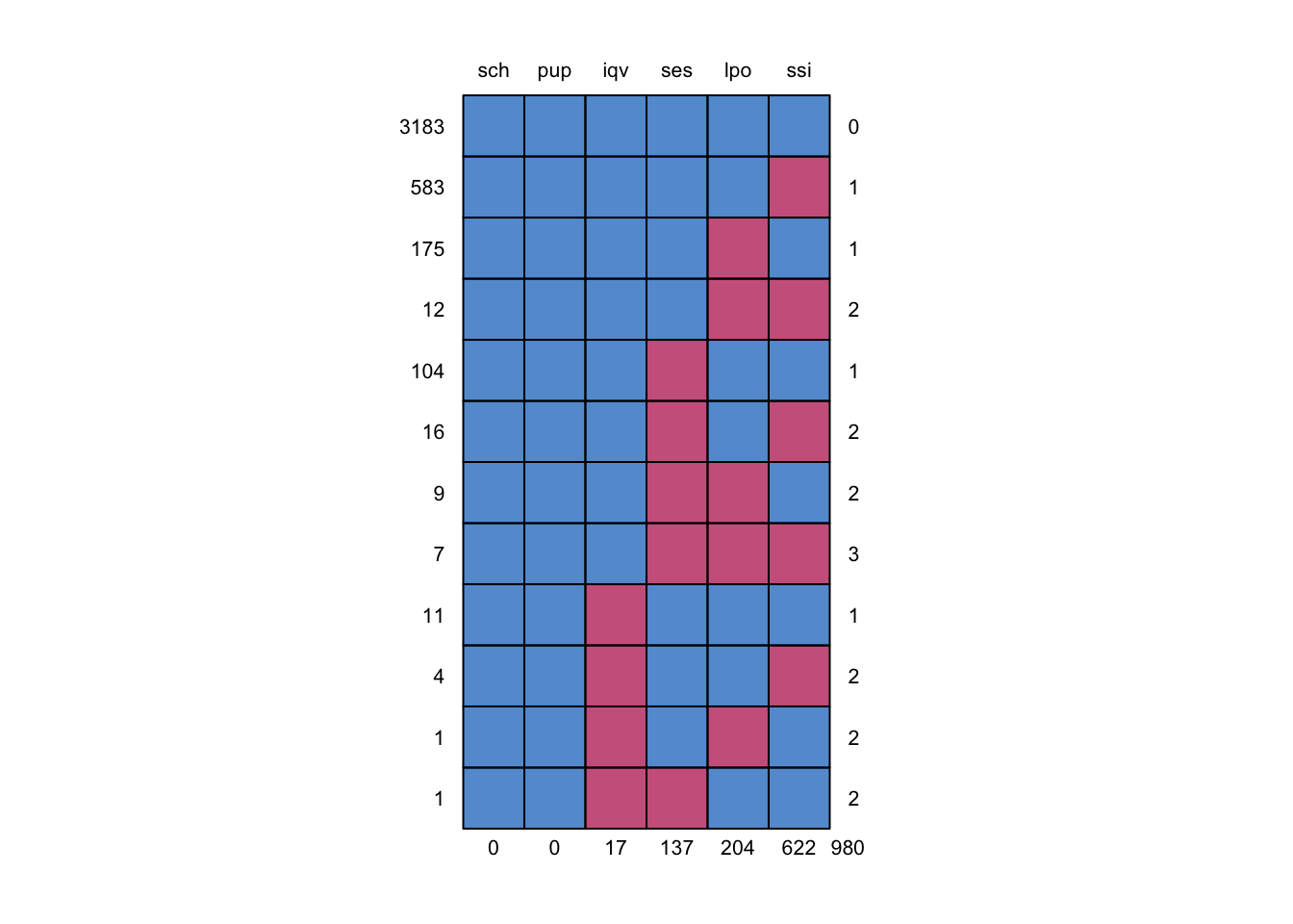
Figure 7.5: Missing data pattern of subset of brandsma data.
Figure 7.5, with the missing data patterns, reveals that there are 3183 (out of 4016) pupils without missing values. For the remaining sample, most have a missing value in just one variable: 583 pupils have only missing ssi, 175 pupils have only missing lpo, 104 pupils have only missing ses and 11 pupils have only missing lpo. The remaining 50 pupils have two or three missing values. The challenge is to perform the analyses from Snijders and Bosker (2012) using the full set with 4016 pupils.
7.10.1 Intercept-only model, missing outcomes
The intercept-only (or empty) model is the simplest multilevel model. We have already imputed the data according to this model in Section 7.6.3. Here we select the imputations according to the 2l.pmm method for further analysis.
d <- brandsma[, c("sch", "lpo")]
pred <- make.predictorMatrix(d)
pred["lpo", "sch"] <- -2
imp <- mice(d, pred = pred, meth = "2l.pmm", m = 10, maxit = 1,
            print = FALSE, seed = 152)
The empty model is fitted to the imputed datasets, and the estimates are pooled as
library(lme4)
fit <- with(imp, lmer(lpo ~ (1 | sch), REML = FALSE))
summary(pool(fit))
estimate std.error statistic df p.value
(Intercept) 40.9 0.322 127 3368 0We may obtain the variance components by the testEstimates() function from mitml:
library(mitml)
testEstimates(as.mitml.result(fit), var.comp = TRUE)$var.comp
Estimate
Intercept~~Intercept|sch 18.021
Residual~~Residual 63.306
ICC|sch 0.222See Example 4.1 in Snijders and Bosker (2012) for the interpretation of the estimates from this model.
7.10.2 Random intercepts, missing level-1 predictor
Let’s now extend the model in order to quantify the impact of IQ on the language score. This random intercepts model with one explanatory variable is defined by
\[ {{\texttt{lpo}}}_{ic} = \gamma_{00} + \gamma_{10} {{\texttt{iqv}}}_{ic} + u_{0c} + \epsilon_{ic}. \tag{7.10} \]
In level notation, the model reads as
\[\begin{align} {{\texttt{lpo}}}_{ic} & = \beta_{0c} + \beta_{1c}{{\texttt{iqv}}}_{ic} + \epsilon_{ic} \tag{7.11}\\ \beta_{0c} & = \gamma_{00} + u_{0c} \tag{7.12}\\ \beta_{1c} & = \gamma_{10} \tag{7.13} \end{align}\]There are missing data in both lpo and iqv. Imputation can be done with both FCS and JM. For FCS my advice is to impute lpo and iqv by 2l.pmm with added cluster means. Adding the cluster means is done here to improve compatibility among the conditional specified imputation models (cf. Section 7.5.1).
d <- brandsma[, c("sch", "lpo", "iqv")]
pred <- make.predictorMatrix(d)
pred["lpo", ] <- c(-2, 0, 3)
pred["iqv", ] <- c(-2, 3, 0)
imp <- mice(d, pred = pred, meth = "2l.pmm", seed = 919,
            m = 10, print = FALSE)
An entry of -2 in the predictor matrix signals the cluster variable, whereas an entry of 3 indicates that the cluster means of the covariates are added as a predictor to the imputation model. Thus, lpo is imputed from iqv and the cluster means of iqv, while iqv is imputed from lpo and the cluster means of lpo. If the residuals are close to normal and the within-cluster error variances are similar, then 2l.pan is also a good choice.
Rescaling the variables as deviations from their mean often helps to improve stability of the estimates. We may rescale lpo to zero-mean by
d$lpo <- as.vector(scale(d$lpo, scale = FALSE))The imputations will also adopt that scale, so we must back-transform the data if we want to analyze the data in the original scale. For the multilevel model with only random intercepts and fixed slopes, rescaling the data to the origin presents no issues since the model is invariant to linear transformations. This is not true when there are random slopes (Hox, Moerbeek, and Van de Schoot 2018, 48). We return to this point in Section 7.10.6.
The JM can create multivariate imputations by the jomoImpute or panImpute methods. We use panImpute here.
fm1 <- lpo + iqv ~ 1 + (1 | sch)
mit <- mitml::panImpute(data = d, formula = fm1, m = 5,
                        silent = TRUE)
which returns as object of class mitml. The panImpute method can also be called from mice by creating one block for all variables as
blk <- make.blocks(d, "collect")
fm2 <- list(collect = fm1)
imp2 <- mice(d, meth = "panImpute", blocks = blk, form = fm2,
             print = FALSE, seed = 711)
This uses a new facility in mice that allows imputation of blocks of variables (cf. Section 4.7.2). The final estimates on the multiply imputed data under model (??) can be calculated (from the 2l.pmm method) as
fit <- with(imp, lmer(lpo ~  iqv + (1 | sch), REML = FALSE))
summary(pool(fit))
estimate std.error statistic df p.value
(Intercept) 40.96 0.2381 172 3305 0
iqv 2.52 0.0525 48 2119 0testEstimates(as.mitml.result(fit), var.comp = TRUE)$var.comp Estimate
Intercept~~Intercept|sch 9.505
Residual~~Residual 40.819
ICC|sch 0.189which produces the estimates for the random intercept model with an effect for IQ with imputed IQ and language scores. See Example 4.2 in Snijders and Bosker (2012) for the interpretation of the parameters.
7.10.3 Random intercepts, contextual model
The ordinary least squares estimator does not distinguish between regressions within groups and between group. This section shows how we can allow for differences in the within- and between-group regressions. The models here parallel Example 4.3 and Table 4.4 in Snijders and Bosker (2012), and row 1 in Table 6 of Grund, Lüdtke, and Robitzsch (2018b).
We continue with the analysis of Section 7.10.2. We extend the complete-data multilevel model by an extra term, as follows:
\[ {{\texttt{lpo}}}_{ic} = \gamma_{00} + \gamma_{01} {{\overline{\texttt{iqv}}}}_{c} + \gamma_{10} {{\texttt{iqv}}}_{ic} + u_{0c} + \epsilon_{ic}.\tag{7.14} \]
In level notation, we get
\[\begin{align} {{\texttt{lpo}}}_{ic} & = \beta_{0c} + \beta_{1c}{{\texttt{iqv}}}_{ic} + \epsilon_{ic} \tag{7.15}\\ \beta_{0c} & = \gamma_{00} + \gamma_{01}{{\overline{\texttt{iqv}}}}_{c} + u_{0c} \tag{7.16}\\ \beta_{1c} & = \gamma_{10} \tag{7.17} \end{align}\]where the variable \({{\overline{\texttt{iqv}}}}_c\) stands for the cluster means of iqv. The model decomposes the contribution of IQ to the regression into a within-group component with parameter \(\gamma_{10}\), and a between-group component with parameter \(\gamma_{01}\). The interest in contextual analysis lies in testing the null hypothesis that \(\gamma_{01} = 0\). Because of this decomposition we need to add the cluster means of lpo and iqv to the imputation model. Remember however that we just did that in the FCS imputation model of Section 7.10.2. Thus, we may use the same set of imputations to perform the within- and between-group regressions.
The following code block adds the cluster means to the imputed data, estimates the model parameters on each set, stores the results in a list, and pools the estimated parameters from the fitted models to get the combined results.
res <- mice::complete(imp, "long") %>%
  group_by(sch, .imp) %>%
  mutate(iqm = mean(iqv)) %>%
  group_by(.imp) %>%
  do(model = lmer(lpo ~ iqv + iqm + (1 | sch),
                  REML = FALSE, data = .)) %>%
  as.list() %>% .[[-1]]
summary(pool(res))
estimate std.error statistic df p.value
(Intercept) 41.02 0.2279 180.04 3056 0.00000000
iqv 2.47 0.0535 46.20 2392 0.00000000
iqm 1.17 0.2571 4.55 667 0.00000562testEstimates(res, var.comp = TRUE)$var.comp Estimate
Intercept~~Intercept|sch 8.430
Residual~~Residual 40.800
ICC|sch 0.171An alternative could have been to use the imp2 object with the imputations under the joint imputation model.
Binary level-1 predictors can be imputed in the same way using one of the methods listed in Table 7.4. It is not yet clear which of the methods should be preferred. No univariate methods yet exist for multi-category variables, but 2l.pmm may be a workable alternative. Categorical variables can be imputed by jomo (Quartagno and Carpenter 2017), jomoImpute (Grund, Robitzsch, and Lüdtke 2018), by latent class analysis (Vidotto 2018), or by Blimp (Keller and Enders 2017).
7.10.4 Random intercepts, missing level-2 predictor
The previous section extended the substantive model by the cluster means. Another extension is to add a measured level-2 predictor. For the sake of illustration we add another variable, religious denomination of the school, as a level-2 predictor. The corresponding complete-data model looks very similar:
\[ {{\texttt{lpo}}}_{ic} = \gamma_{00} + \gamma_{01} {{\texttt{den}}}_{c} + \gamma_{10}{{\texttt{iqv}}}_{ic} + u_{0c} + \epsilon_{ic}. \tag{7.18} \]
In level notation, we get
\[\begin{align} {{\texttt{lpo}}}_{ic} & = \beta_{0c} + \beta_{1c}{{\texttt{iqv}}}_{ic} + \epsilon_{ic} \tag{7.19}\\ \beta_{0c} & = \gamma_{00} + \gamma_{01}{{\texttt{den}}}_{c} + u_{0c} \tag{7.20}\\ \beta_{1c} & = \gamma_{10} \tag{7.21} \end{align}\]The missing values occur in lpo, iqv and den. The difference with model (7.14) is that den is a measured variable, so the value is identical for all members of the same cluster. If den is missing, it is missing for the entire cluster. Imputing a missing level-2 predictor is done by forming an imputation model at the cluster level.
Imputation can be done with both FCS and JM (cf. Table 6, row 3 in Grund, Lüdtke, and Robitzsch (2018b)). For FCS, the advice is to include aggregates of all level-1 variables into the cluster level imputation model. Methods 2lonly.norm and 2lonly.pmm add the means of all level-1 variables as predictors, and subsequently follow the rules for single-level imputation at level-2.
The following code block imputes missing values in the 2-level predictor den. For reasons of simplicity, I have used 2lonly.pmm, so imputations adhere to original four-point scale. This use of predictive mean matching rests on the assumption that the relative frequency of the denomination categories changes with a linear function. Alternatively, one might opt for a true categorical method to impute den, which would introduce additional parameters into the imputation model.
d <- brandsma[, c("sch", "lpo", "iqv", "den")]
meth <- make.method(d)
meth[c("lpo", "iqv", "den")] <- c("2l.pmm", "2l.pmm",
                                  "2lonly.pmm")
pred <- make.predictorMatrix(d)
pred["lpo", ] <- c(-2, 0, 3, 1)
pred["iqv", ] <- c(-2, 3, 0, 1)
pred["den", ] <- c(-2, 1, 1, 0)
imp <- mice(d, pred = pred, meth = meth, seed = 418,
            m = 10, print = FALSE)
The following statements address the same imputation task as a joint model by jomoImpute:
d$den <- as.factor(d$den)
fml <- list(lpo + iqv ~ 1 + (1 | sch), den ~ 1)
mit <- mitml::jomoImpute(data = d, formula = fml, m = 10,
                         silent = TRUE)
An alternative is to call jomoImpute() from mice, as follows:
blk <- make.blocks(d, "collect")
fm2 <- list(collect = fml)
imp2 <- mice(d, meth = "jomoImpute", blocks = blk, form = fm2,
             print = FALSE, seed = 418, maxit = 1,
             m = 10, n.burn = 100)
Because mice calls jomoImpute per replication, the latter method can be slow because the entire burn-in sequence is re-run for every call. Inspection of the trace lines revealed that autocorrelations were low and convergence was quick. To improve speed, the number of burn-in iterations was lowered from n.burn = 5000 (default) to n.burn = 100. The total number of iterations was set as maxit = 1, since all variables were members of the same block.
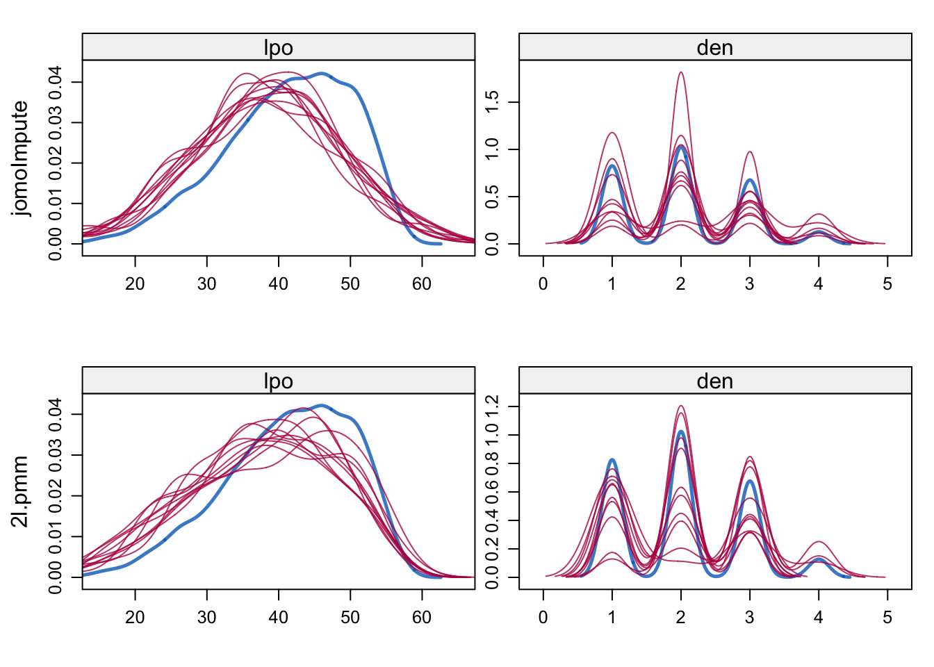
Figure 7.6: Density plots for language score and denomination after jomoImpute (top) and 2l.pmm (bottom).
Figure 7.6 shows the density plots of the observed and imputed data after applying the joint mixed normal/categorical model, and after predictive mean matching. Both methods handle categorical data, so the figures for den have multiple modes. The imputations of lpo under JM and FCS are very similar, with jomoImpute slightly closer to normality. The complete-data analysis on the multiply imputed data can be fitted as
fit <- with(imp, lmer(lpo ~ 1 + iqv + as.factor(den)
                      + (1 | sch), REML = FALSE))
summary(pool(fit))
estimate std.error statistic df p.value
(Intercept) 40.071 0.4549 88.09 187 0.000000
iqv 2.516 0.0532 47.34 1242 0.000000
as.factor(den)2 2.041 0.5925 3.45 430 0.000589
as.factor(den)3 0.234 0.6519 0.36 285 0.719226
as.factor(den)4 1.843 1.1642 1.58 1041 0.113706testEstimates(as.mitml.result(fit), var.comp = TRUE)$var.comp Estimate
Intercept~~Intercept|sch 8.621
Residual~~Residual 40.761
ICC|sch 0.1757.10.5 Random intercepts, interactions
The random intercepts model may have predictors at level-1, at level-2, and possibly interactions within and/or across levels. A level-2 variable can be a level-1 aggregate (e.g., as in Section 7.10.3), or a measured level-2 variable (as in Section 7.10.4). Missing values in the measured variables will propagate through the interaction terms. This section suggests imputation methods for the model with random intercepts and interactions.
We continue with the brandsma data, and include three types of multiplicative interactions among the predictors into the model:
a level-1 interaction, e.g., \({{\texttt{iqv}}}_{ic} \times {{\texttt{sex}}}_{ic}\);
a cross-level interaction, e.g., \({{\texttt{sex}}}_{ic} \times {{\texttt{den}}}_c\);
a level-2 interaction, e.g., \({{\overline{\texttt{iqv}}}}_c \times {{\texttt{den}}}_c\).
The extended model in composite notation is defined by:
\[\begin{align} {{\texttt{lpo}}}_{ic} = & \gamma_{00} + \gamma_{10}{{\texttt{iqv}}}_{ic} + \gamma_{20}{{\texttt{sex}}}_{ic} + \gamma_{30}{{\texttt{iqv}}}_{ic}{{\texttt{sex}}}_{ic} + \gamma_{40}{{\texttt{sex}}}_{ic}{{\texttt{den}}}_c + \\ & \gamma_{01}{{\overline{\texttt{iqv}}}}_c + \gamma_{02}{{\texttt{den}}}_c + \gamma_{03}{{\overline{\texttt{iqv}}}}_c{{\texttt{den}}}_c + u_{0c} + \epsilon_{ic}. \end{align}\]In level notation, the model is
\[\begin{align} {{\texttt{lpo}}}_{ic} & = \beta_{0c} + \beta_{1c}{{\texttt{iqv}}}_{ic} + \beta_{2c}{{\texttt{sex}}}_{ic} + \beta_{3c}{{\texttt{iqv}}}_{ic}{{\texttt{sex}}}_{ic} + \beta_{4c}{{\texttt{sex}}}_{ic}{{\texttt{den}}}_c + \epsilon_{ic}\\ \beta_{0c} & = \gamma_{00} + \gamma_{01}{{\overline{\texttt{iqv}}}}_c + \gamma_{02}{{\texttt{den}}}_c + \gamma_{03}{{\overline{\texttt{iqv}}}}_c{{\overline{\texttt{den}}}}_c + u_{0c}\\ \beta_{1c} & = \gamma_{10}\\ \beta_{2c} & = \gamma_{20}\\ \beta_{3c} & = \gamma_{30}\\ \beta_{4c} & = \gamma_{40}\\ \end{align}\]How should we impute the missing values in lpo, iqv, sex and den, and obtain valid estimates for the interaction term? Grund, Lüdtke, and Robitzsch (2018b) recommend FCS with passive imputation of the interaction terms. As a first step, we initialize a number of derived variables. ` `
d <- brandsma[, c("sch", "lpo", "iqv", "sex", "den")]
d <- data.frame(d, lpm = NA, iqm = NA, sxm = NA,
                iqd = NA, lpd = NA,
                iqd.sex = NA, lpd.sex = NA, iqd.lpd = NA,
                iqd.den = NA, sex.den = NA, lpd.den = NA,
                iqm.den = NA, sxm.den = NA, lpm.den = NA)
The new variables lpm, iqm and sxm will hold the cluster means of lpo, iqv and sex, respectively. Variables iqd and lpd will hold the values of iqv and lpo in deviations from their cluster means. Variables iqd.sex, lpd.sex and iqd.lpd are two-way interactions of level-1 variables scaled as deviations from the cluster means. Variables iqd.den, sex.den and lpd.den are cross-level interactions. Finally, iqm.den, sxm.den and lpm.den are interactions at level-2. For simplicity, we ignore further level-2 interactions between iqm, sxm and lpm.
The idea is that we impute lpo, iqv, sex and den, and update the other variables accordingly. Level-1 variables are imputed by two-level predictive mean matching, and include as predictor the other level-1 variables, the two-way interactions between the other level-1 variables (in deviations from their group means), level-2 variables, and cross-level interactions.
# level-1 variables
meth <- make.method(d)
meth[c("lpo", "iqv", "sex")] <- "2l.pmm"

pred <- make.predictorMatrix(d)
pred[,] <- 0
pred[, "sch"] <- -2
codes <- c(3, 3, rep(1, 6))
pred["lpo", c("iqv", "sex", "iqd.sex", "sex.den", "iqd.den",
              "den", "iqm.den", "sxm.den")] <- codes
pred["iqv", c("lpo", "sex", "lpd.sex", "sex.den", "lpd.den",
              "den", "lpm.den", "sxm.den")] <- codes
pred["sex", c("lpo", "iqv", "iqd.lpd", "lpd.den", "iqd.den",
              "den", "iqm.den", "lpm.den")] <- codes
Level-2 variables are imputed by predictive mean matching on level 2, using as predictors the aggregated level-1 variables, and the aggregated two-way interactions of the level-1 variables, and - if available - other level-2 variables and their two-way interactions.
# level-2 variables
meth["den"] <- "2lonly.pmm"
pred["den", c("lpo", "iqv", "sex",
              "iqd.sex", "lpd.sex", "iqd.lpd")] <- 1
The transpose of the relevant entries of the predictor matrix illustrates the symmetric structure of the imputation model.
        lpo iqv sex den
sch      -2  -2  -2  -2
lpo       0   3   3   1
iqv       3   0   3   1
sex       3   3   0   1
den       1   1   1   0
iqd.sex   1   0   0   1
lpd.sex   0   1   0   1
iqd.lpd   0   0   1   1
iqd.den   1   0   1   0
sex.den   1   1   0   0
lpd.den   0   1   1   0
iqm.den   1   0   1   0
sxm.den   1   1   0   0
lpm.den   0   1   1   0
The entries corresponding to the level-1 predictors are coded with a 3, indicating that both the original values as well as the cluster means of the predictor are included into the imputation model. Interactions are coded with a 1. One could also code these with a 3, in order to improve compatibility, but this is not done here because the imputation model becomes too heavy. Because we cannot have the same variable appearing at both sides of the equation, any interaction terms involving the target have been deleted from the conditional imputation models.
The specification above defines the imputation model for the variables in the data. All other variables (e.g., cluster means, interactions) are calculated on-the-fly by passive imputation. The code below centers iqm and lpo relative to their cluster means.
# derive group means
meth[c("iqm", "sxm", "lpm")] <- "2l.groupmean"
pred[c("iqm", "sxm", "lpm"), c("iqv", "sex", "lpo")] <- diag(3)

# derive deviations from cluster mean
meth["iqd"] <- "~ I(iqv - iqm)"
meth["lpd"] <- "~ I(lpo - lpm)"
The 2l.groupmean method from the miceadds package returns the cluster mean pertaining to each observation. Centering on the cluster means is widely practiced, but significantly alters the multilevel model. In the context of imputation, centering on the cluster means often enhances stability and robustness of models to generate imputations, especially if interactions are involved. When the complete-data model uses cluster centering, then the imputation model should also do so. See Section 7.5.1 for more details.
The next block of code specifies the interaction effects, by means of passive imputation.
# derive interactions
meth["iqd.sex"] <- "~ I(iqd * sex)"
meth["lpd.sex"] <- "~ I(lpd * sex)"
meth["iqd.lpd"] <- "~ I(iqd * lpd)"
meth["iqd.den"] <- "~ I(iqd * den)"
meth["sex.den"] <- "~ I(sex * den)"
meth["lpd.den"] <- "~ I(lpd * den)"
meth["iqm.den"] <- "~ I(iqm * den)"
meth["sxm.den"] <- "~ I(sxm * den)"
meth["lpm.den"] <- "~ I(lpm * den)"
The visit sequence specified below updates the relevant derived variables after any of the measured variables is imputed, so that interactions are always in sync. The specification of the imputation model is now complete, so it can be run with mice().
visit <- c("lpo", "lpm", "lpd",
           "lpd.sex", "iqd.lpd", "lpd.den", "lpm.den",
           "iqv", "iqm", "iqd",
           "iqd.sex", "iqd.lpd", "iqd.den", "iqm.den",
           "sex", "sxm",
           "iqd.sex", "lpd.sex", "sex.den", "sxm.den",
           "den", "iqd.den", "sex.den", "lpd.den",
           "iqm.den", "sxm.den", "lpm.den")

imp <- mice(d, pred = pred, meth = meth, seed = 188,
            visit = visit, m = 10, print = FALSE,
            allow.na = TRUE)
The analysis of the imputed data according to the specified model first transforms den into a categorical variable, and then fits and pools the mixed model.
long <- mice::complete(imp, "long", include = TRUE)
long$den <- as.factor(long$den)
imp2 <- as.mids(long)
fit <- with(imp2, lmer(lpo ~ 1 + iqv*sex + iqm*den + sex*den
                      + (1 | sch), REML = FALSE))
summary(pool(fit))
estimate std.error statistic df p.value
(Intercept) 39.371 0.4620 85.228 660 0.00e+00
iqv 2.540 0.0742 34.222 391 0.00e+00
sex 2.503 0.3785 6.613 873 4.95e-11
iqm 1.497 0.4336 3.453 271 5.68e-04
den2 1.795 0.6245 2.875 444 4.09e-03
den3 -0.613 0.6742 -0.909 391 3.63e-01
den4 1.935 1.4749 1.312 823 1.90e-01
iqv:sex -0.139 0.1084 -1.284 192 1.99e-01
iqm:den2 -0.400 0.6503 -0.615 304 5.39e-01
iqm:den3 -0.757 0.5757 -1.315 968 1.89e-01
iqm:den4 -1.841 1.4083 -1.307 1403 1.91e-01
sex:den2 -0.653 0.5014 -1.302 1372 1.93e-01
sex:den3 0.787 0.5742 1.371 433 1.71e-01
sex:den4 -0.370 1.0052 -0.368 1811 7.13e-017.10.6 Random slopes, missing outcomes and predictors
So far our examples were restricted to models with random intercepts. We continue here with the contextual model that includes random slopes for IQ (cf. Example 5.1 in Snijders and Bosker (2012)). Section 7.10.3 showed how to impute the contextual model. Including random slopes extends the complete-data model as
\[ {{\texttt{lpo}}}_{ic} = \gamma_{00} + \gamma_{01}{{\overline{\texttt{iqv}}}}_{c} + \gamma_{10}{{\texttt{iqv}}}_{ic} + u_{0c} + u_{1c} {{\texttt{iqv}}}_{ic} + \epsilon_{ic} \tag{7.22} \]
When expressed in level notation, the model is
\[\begin{align} {{\texttt{lpo}}}_{ic} & = \beta_{0c} + \beta_{1c}{{\texttt{iqv}}}_{ic} + \epsilon_{ic} \tag{7.23}\\ \beta_{0c} & = \gamma_{00} + \gamma_{01}{{\overline{\texttt{iqv}}}}_{c} + u_{0c} \tag{7.24}\\ \beta_{1c} & = \gamma_{10} + u_{1c} \tag{7.25} \end{align}\]The addition of the term \(u_{1c}\) to the equation for \(\beta_{1c}\) allows for \(\beta_{1c}\) to vary over clusters, hence the name “random slopes”.
Missing data may occur in lpo and iqv. Enders, Mistler, and Keller (2016) and Grund, Lüdtke, and Robitzsch (2018b) recommend FCS for this problem. The procedure is almost identical to that in Section 7.10.2, but now including both the cluster means and random slopes into the imputation model.
d <- brandsma[, c("sch", "lpo", "iqv")]
d$lpo <- as.vector(scale(d$lpo, scale = FALSE))
pred <- make.predictorMatrix(d)
pred["lpo", ] <- c(-2, 0, 4)
pred["iqv", ] <- c(-2, 4, 0)
pred
sch lpo iqv
sch 0 1 1
lpo -2 0 4
iqv -2 4 0imp <- mice(d, pred = pred, meth = "2l.pmm", seed = 441,
m = 10, print = FALSE, maxit = 20)The entry of 4 at cell (lpo, iqv) in the predictor matrix adds three variables to the imputation model for lpo: the value of iqv, the cluster means of iqv and the random slopes of iqv. Conversely, imputing iqv adds the three covariates: the values of lpo, the cluster means of lpo and the random slopes of lpo.
The iqv variable had zero mean in the data, so this could be imputed right away, but lpo needs to be centered around the grand mean in order to reduce the large number of warnings about unstable estimates. It is known that the random slopes model is not invariant to a shift in origin in the predictors (Hox, Moerbeek, and Van de Schoot 2018), so we may wonder what the effect of centering on the grand mean will be on the quality of the imputations. See Kreft, De Leeuw, and Aiken (1995) and Enders and Tofighi (2007) for discussions on the effects of centering in multilevel models. In imputation, we generally have no desire to attach a meaning to the parameters of the imputation model, so centering on the grand mean is often beneficial. Grand-mean centering implies a little extra work because we must back-transform the data if we want the values in the original scale. What remains is that rescaling improves speed and stability, so for the purpose of imputation I recommend to scale level-1 variables in deviations from their means.
The following code block unfolds the mids object, adds the IQ cluster means, restores the rescaling of lpo, and estimates and combines the parameters of the random slopes model.
imp2 <- mice::complete(imp, "long", include = TRUE) %>%
  group_by(sch) %>%
  mutate(iqm = mean(iqv, na.rm = TRUE),
         lpo = lpo + mean(brandsma$lpo, na.rm = TRUE)) %>%
  as.mids()
fit <- with(imp2, lmer(lpo ~  iqv + iqm + (1 + iqv | sch),
                       REML = FALSE))
summary(pool(fit))
estimate std.error statistic df p.value
(Intercept) 41.061 0.228 179.85 3508 0.000000
iqv 2.495 0.063 39.63 1511 0.000000
iqm 0.975 0.261 3.74 620 0.000185testEstimates(as.mitml.result(fit), var.comp = TRUE)$var.comp Estimate
Intercept~~Intercept|sch 8.591
Intercept~~iqv|sch -0.781
iqv~~iqv|sch 0.188
Residual~~Residual 39.791
ICC|sch 0.178See Example 5.1 in Snijders and Bosker (2012) for the interpretation of these model parameters. Interestingly, if we don’t restore the mean of lpo, the estimated intercept represents the average difference between the observed and imputed language scores. Its value here is -0.271 (not shown), so on average pupils without a language test score a little lower than pupils with a score. The difference is not statistically significant (\(p = 0.23\)).
7.10.7 Random slopes, interactions
Random slopes models may also include interactions among level-1 predictors, among level-2 predictors, and between level-1 and level-2 predictor (cross-level interactions). This section concentrates on imputation under the model described in Example 5.3 of Snijders and Bosker (2012). This is a fairly elaborate model that can best be understood in level notation:
\[\begin{align} {{\texttt{lpo}}}_{ic} & = \beta_{0c} + \beta_{1c}{{\texttt{iqv}}}_{ic} + \beta_{2c}{{\texttt{ses}}}_{ic} + \beta_{3c}{{\texttt{iqv}}}_{ic}{{\texttt{ses}}}_{ic} + \epsilon_{ic} \tag{7.26}\\ \beta_{0c} & = \gamma_{00} + \gamma_{01}{{\overline{\texttt{iqv}}}}_c + \gamma_{02}{{\overline{\texttt{ses}}}}_c + \gamma_{03}{{\overline{\texttt{iqv}}}}_c{{\overline{\texttt{ses}}}}_c + u_{0c} \tag{7.27}\\ \beta_{1c} & = \gamma_{10} + \gamma_{11}{{\overline{\texttt{iqv}}}}_c + \gamma_{12}{{\overline{\texttt{ses}}}}_c + u_{1c} \tag{7.28}\\ \beta_{2c} & = \gamma_{20} + \gamma_{21}{{\overline{\texttt{iqv}}}}_c + \gamma_{22}{{\overline{\texttt{ses}}}}_c + u_{2c} \tag{7.29}\\ \beta_{3c} & = \gamma_{30} \tag{7.30} \end{align}\]which can be reorganized into composite notation as:
\[\begin{align} {{\texttt{lpo}}}_{ic} = & \gamma_{00} + \gamma_{10}{{\texttt{iqv}}}_{ic} + \gamma_{20}{{\texttt{ses}}}_{ic} + \gamma_{30}{{\texttt{iqv}}}_{ic}{{\texttt{ses}}}_{ic} + \\ & \gamma_{01}{{\overline{\texttt{iqv}}}}_c + \gamma_{02}{{\overline{\texttt{ses}}}}_c + \\ & \gamma_{11}{{\texttt{iqv}}}_{ic}{{\overline{\texttt{iqv}}}}_c + \gamma_{12}{{\texttt{iqv}}}_{ic}{{\overline{\texttt{ses}}}}_c + \gamma_{21}{{\texttt{ses}}}_{ic}{{\overline{\texttt{iqv}}}}_c + \gamma_{22}{{\texttt{ses}}}_{ic}{{\overline{\texttt{ses}}}}_c + \\ & \gamma_{03}{{\overline{\texttt{iqv}}}}_c{{\overline{\texttt{ses}}}}_c + \\ & u_{0c} + u_{1c} {{\texttt{iqv}}}_{ic} + u_{2c} {{\texttt{ses}}}_{ic} + \\ & \epsilon_{ic}. \end{align}\]Although this expression may look somewhat horrible, it clarifies that the expected value of lpo depends on the following terms:
the level-1 variables \({{\texttt{iqv}}}_{ic}\) and \({{\texttt{ses}}}_{ic}\);
the level-1 interaction \({{\texttt{iqv}}}_{ic}{{\texttt{ses}}}_{ic}\);
the cluster means \({{\overline{\texttt{iqv}}}}_c\) and \({{\overline{\texttt{ses}}}}_c\);
the within-variable cross-level interactions \({{\texttt{iqv}}}_{ic}{{\overline{\texttt{iqv}}}}_c\) and \({{\texttt{ses}}}_{ic}{{\overline{\texttt{ses}}}}_c\);
the between-variable cross-level interactions \({{\texttt{iqv}}}_{ic}{{\overline{\texttt{ses}}}}_c\) and \({{\texttt{ses}}}_{ic}{{\overline{\texttt{iqv}}}}_c\);
the level-2 interaction \({{\overline{\texttt{iqv}}}}_c{{\overline{\texttt{ses}}}}_c\);
the random intercepts;
the random slopes for
iqvandses.
All terms need to be included into the imputation model for lpo. Univariate imputation models for iqv and ses can be specified along the same principles by reversing the roles of outcome and predictor. As a first step, let us pad the data with the set of all relevant interactions from model (??).
d <- brandsma[, c("sch", "lpo", "iqv", "ses")]
d$lpo <- as.vector(scale(d$lpo, scale = FALSE))
d <- data.frame(d,
                iqv.ses = NA, ses.lpo = NA, iqv.lpo = NA,
                lpm = NA, iqm = NA, sem = NA,
                iqv.iqm = NA, ses.sem = NA, lpo.lpm = NA,
                iqv.sem = NA, iqv.lpm = NA,
                ses.iqm = NA, ses.lpm = NA,
                lpo.iqm = NA, lpo.sem = NA,
                iqm.sem = NA, lpm.sem = NA, iqm.lpm = NA)
Here iqv.ses represents the multiplicative interaction term for iqv and ses, and lpm represents the cluster means of lpo, and so on. Imputation models for lpo, iqv and ses are specified by setting the relevant entries in the transformed predictor matrix as follows:
        lpo iqv ses
sch      -2  -2  -2
lpo       0   3   3
iqv       3   0   3
ses       3   3   0
iqv.ses   1   0   0
ses.lpo   0   1   0
iqv.lpo   0   0   1
iqv.iqm   1   0   1
ses.sem   1   1   0
lpo.lpm   0   1   1
iqv.sem   1   0   0
iqv.lpm   0   0   1
ses.iqm   1   0   0
ses.lpm   0   1   0
lpo.iqm   0   0   1
lpo.sem   0   1   0
iqm.sem   1   0   0
lpm.sem   0   1   0
iqm.lpm   0   0   1
The model for lpo is almost equivalent to model (??). According to the model, both cluster means and random effects should be included, thus values pred[lpo, c(iqv, ses)] should be coded as a 4, and not as a 3. However, the cluster means and random effects are almost linearly dependent, which causes slow convergence and unstable estimates in the imputation model. These problems disappear when only the cluster means are included as covariates. An alternative is to scale the predictors in deviations from the cluster means, as was done in Section 7.10.5. This circumvents many of the computational issues of raw-scored variables, and the parameters are easier to interpret.
The specifications for iqv and ses correspond to the inverted models. Inverting the random slope model produces reasonable estimates for the fixed effect and the intercept variance, but estimates of the slope variance can be unstable and biased, especially in small samples (Grund, Lüdtke, and Robitzsch 2016a). Unless the interest is in the slope variance (for which listwise deletion appears to be better), using FCS by inverting the random slope model is the currently preferred method to account for differences in slopes between clusters.
Next, we need to specify the derived variables. The cluster means are updated by the 2l.groupmean method.
meth[c("iqm", "sem", "lpm")] <- "2l.groupmean"
pred[c("iqm", "sem", "lpm"), ] <- 0
pred["iqm", c("sch", "iqv")] <- c(-2, 1)
pred["sem", c("sch", "ses")] <- c(-2, 1)
pred["lpm", c("sch", "lpo")] <- c(-2, 1)
The level-1 interactions are updated by passive imputation.
meth["iqv.ses"] <- "~ I(iqv * ses)"
meth["iqv.lpo"] <- "~ I(iqv * lpo)"
meth["ses.lpo"] <- "~ I(ses * lpo)"
The remaining interactions are updated by passive imputation in an analogous way (code not shown).
The visit sequence updates the derived variables that depend on the target variable.
visit <- c("lpo", "iqv.lpo", "ses.lpo",
           "lpm", "lpo.lpm", "iqv.lpm", "ses.lpm",
           "lpo.iqm", "lpo.sem", "iqm.lpm", "lpm.sem",
           "iqv", "iqv.ses", "iqv.lpo",
           "iqm", "iqv.iqm", "iqv.sem", "iqv.lpm",
           "ses.iqm", "lpo.iqm", "iqm.sem", "iqm.lpm",
           "ses", "iqv.ses", "ses.lpo",
           "sem", "ses.sem", "iqv.sem", "ses.iqm",
           "ses.lpm", "lpo.sem", "iqm.sem", "lpm.sem")

imp <- mice(d, pred = pred, meth = meth, seed = 211,
            visit = visit, m = 10, print = FALSE, maxit = 10,
            allow.na = TRUE)
The model can now be fitted to the full data as
fit <- with(imp, lmer(lpo ~ iqv * ses + iqm * sem +
                  iqv * iqm + iqv * sem +
                  ses * iqm + ses * sem + (1 + ses + iqv | sch),
REML = FALSE))summary(pool(fit)) estimate std.error statistic df p.value
(Intercept) 0.1801828 0.25242 0.7138 2584 0.47538
iqv 2.2421838 0.06205 36.1369 2619 0.00000
ses 0.1709524 0.01238 13.8100 695 0.00000
iqm 0.7675273 0.30994 2.4763 502 0.01332
sem -0.0921057 0.04372 -2.1066 2756 0.03522
iqv:ses -0.0172118 0.00631 -2.7261 370 0.00644
iqm:sem -0.1167091 0.03758 -3.1060 807 0.00191
iqv:iqm -0.0631837 0.07480 -0.8446 3675 0.39836
iqv:sem 0.0045330 0.01371 0.3307 487 0.74086
ses:iqm 0.0171123 0.01882 0.9095 268 0.36317
ses:sem 0.0000898 0.00235 0.0382 470 0.96953testEstimates(as.mitml.result(fit), var.comp = TRUE)$var.comp Estimate
Intercept~~Intercept|sch 7.93524
Intercept~~ses|sch -0.00920
Intercept~~iqv|sch -0.75078
ses~~ses|sch 0.00114
ses~~iqv|sch -0.00830
iqv~~iqv|sch 0.16489
Residual~~Residual 37.78840
ICC|sch 0.17355The estimates are quite close to Table 5.3 in Snijders and Bosker (2012). These authors continue with simplifying the model. The same set of imputations can be used for these simpler models since the imputation model is more general than the substantive models.
7.10.8 Recipes
The term “cookbook statistics” is sometimes used to refer to thoughtless and rigid applications of statistical procedures. Minute execution of a sequence of steps won’t earn you a Nobel Prize, but a good recipe will enable you to produce a decent meal from ingredients that you may not have seen before. The recipes given here are intended to assist you to create a decent set of imputations for multilevel data.
| Recipe for a level-1 target | |
|---|---|
| 1. | Define the most general analytic model to be applied to imputed data |
| 2. | Select a 2l method that imputes close to the data |
| 3. | Include all level-1 variables |
| 4. | Include the disaggregated cluster means of all level-1 variables |
| 5. | Include all level-1 interactions implied by the analytic model |
| 6. | Include all level-2 predictors |
| 7. | Include all level-2 interactions implied by the analytic model |
| 8. | Include all cross-level interactions implied by the analytic model |
| 9. | Include predictors related to the missingness and the target |
| 10. | Exclude any terms involving the target |
| Recipe for a level-2 target | |
|---|---|
| 1. | Define the most general analytic model to be applied to imputed |
| data | |
| 2. | Select a 2lonly method that imputes close to the data |
| 3. | Include the cluster means of all level-1 variables |
| 4. | Include the cluster means of all level-1 interactions |
| 5. | Include all level-2 predictors |
| 6. | Include all interactions of level-2 variables |
| 7. | Include predictors related to the missingness and the target |
| 8. | Exclude any terms involving the target |
Tables 7.5 and 7.6 contains two recipes for imputing multilevel data. There are separate recipes for level-1 and level-2 data. The recipes follow the inclusive strategy advocated by Collins, Schafer, and Kam (2001), and extend the predictor specification strategy in Section 6.3.2 to multilevel data. Including all two-way (or higher-order) interactions may quickly inflate the number of parameters in the model, especially for categorical data, so some care is needed in selecting the interactions that seem most important to the application at hand.
Sections 7.10.1 to 7.10.7 demonstrated applications of these recipes for a variety of multilevel models. One very important source of information was not yet included. For clarity, all procedures were restricted to the subset of data that was actually used in the model. This strategy is not optimal in general because it fails to include potentially auxiliary information that is not modeled. For example, the brandsma data also contains the test scores from the same pupils taken one year before the outcome was measured. This score is highly correlated to the outcome, but it was not part of the model and hence not used for imputation. Of course, one could extend the substantive model (e.g., include the pre-test score as a covariate), but this affects the interpretation and may not correspond to the question of scientific interest. A better way is to include these variables only into the imputation model. This will decrease the between-imputation variability and hence lead to sharper statistical inferences. Including extra predictive variables is left as an exercise for the reader.
The procedure in Section 7.10.7 may be a daunting task when the number of variables grows, especially keeping track of all required interaction effects. The whole process can be automated, but currently there is no software that will perform these steps behind the screen. This may be a matter of time. In general, it is good to be aware of the steps taken, so specification by hand could also be considered an advantage.
Monitoring convergence is especially important for models with many random slopes. Warnings from the underlying multilevel routines may indicate over-specification of the model, for example, with a too large number of parameters. The imputer should be attentive to such messages by reducing the complexity of imputation model in the light of the analytic model. In multilevel modeling, overparameterization occurs almost always in the variance part of the model. Reducing the number of random slopes, or simplifying the level-2 model structure could help to reduce computational complexity.