8.4 Generating imputations by FCS
We return to the data in Table 8.1. Suppose that the assignment mechanism depends on age only, where patients up to age 70 years are allocated to the new surgery with a probability of 0.75, and older patients are assigned the new surgery with a probability of 0.5. The next code creates the data that we might see after the study. John, Caren and Joyce (mean age 70) were assigned to the new surgery, whereas the other five (mean age 75) obtained standard surgery.
ideal <- data.frame(
  x = c(68, 76, 66, 81, 70, 72, 81, 72),
  y1 = c(14, 0, 1, 2, 3, 1, 10, 9),
  y0 = c(13, 6, 4, 5, 6, 6, 8, 8),
  row.names = c("John", "Caren", "Joyce", "Robert",
                "Ruth", "Nick", "Peter", "Torey")
)

# assign first three units to trt
data <- ideal
data[1:3, "y0"] <- NA
data[4:8, "y1"] <- NA
8.4.1 Naive FCS
We are interested in obtaining estimates of \(\tau_i\) from the data. We generate imputations by assuming a normal distribution for the potential outcomes y1 and y0. Let us for the moment ignore the impact of age on assignment. The next code block represents a naive first try to impute the missing values.
library(mice)
data2 <- data[, -1]
imp <- mice(data2, method = "norm", seed = 188, print = FALSE)
Warning: Number of logged events: 7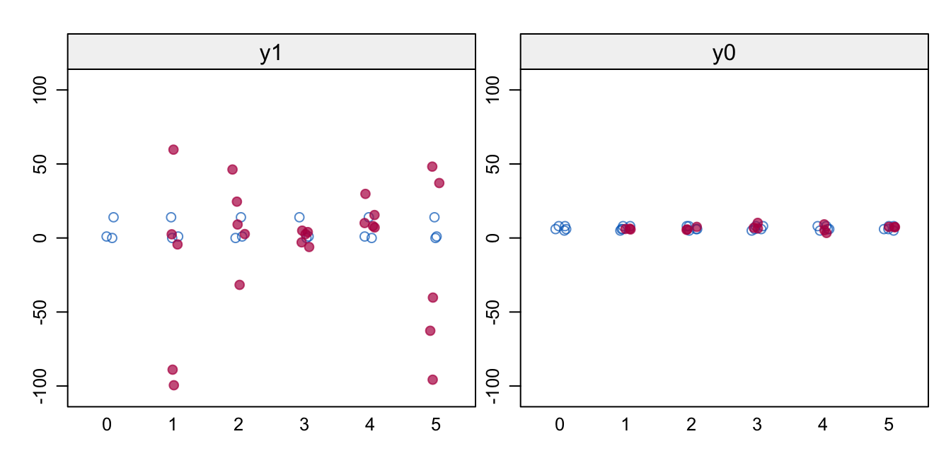
Figure 8.1: Naive FCS. Stripplot of \(m=5\) of observed (blue) and imputed (red) data for the potential outcomes y1 and y0. Imputations are odd, especially for y1.
Figure 8.1 shows the values of the observed and imputed data of the potential outcomes. The imputations look very bad, especially for y1. The spread is much larger than in the data, resulting in illogical negative values and implausible high values. The problem is that there are no persons for which y1 and y0 are jointly observed, so the relation between y1 and y0 is undefined. We may see this clearly from the correlations \(\rho(Y(0),Y(1))\) between the two potential outcomes in each imputed dataset.
sapply(mice::complete(imp, "all"), function(x) cor(x$y1, x$y0)) 1 2 3 4 5
-0.994 -0.552 0.952 0.594 -0.558 The \(\rho\)’s are all over the place, signaling that the correlation \(\rho(Y(0),Y(1))\) is not identified from the data in y1 and y0, a typical finding for the file matching missing data pattern.
8.4.2 FCS with a prior for \(\rho\)
We stabilize the solution by specifying a prior for \(\rho(Y(0),Y(1))\). The data are agnostic to the specification, in the sense that the data will not contradict or support a given value. However, some \(\rho\)’s will be more plausible than others in the given scientific context. A high value for \(\rho\) implies that the variation between the different \(\tau_i\) is relatively small. The extreme case \(\rho = 1\) corresponds to the assumption of homogeneous treatment effects. Setting lower values (e.g., \(\rho = 0\)) allows for substantial heterogeneity in treatment effects. If we set the extreme \(\rho = -1\), we expect that the treatment would entirely reverse the order of units, so the unit with the maximum outcome under treatment will have the minimum outcome under control, and vice versa. It is hard to imagine interventions for which that would be realistic.
The \(\rho\) parameter can act as a tuning knob regulating the amount of heterogeneity in the imputation. In my experience, \(\rho\) has to be set at fairly high value, say in the range 0.9 – 0.99. The correlation in Table 8.1 is 0.9, which allows for fairly large differences in \(\tau_i\), here from \(-6\) years to \(+2\) years.
The specification \(\rho\) in mice can be a little tricky, and is most easily achieved by appending hypothetical extra cases to the data with both y1 and y0 observed given the specified correlation. Following Imbens and Rubin (2015, 165) we assume a bivariate normal distribution for the potential outcomes:
\[ \left( \begin{array}{c} Y_i(0) \\ Y_i(1) \end{array}\right) \bigg | \theta \sim N \left( \left( \begin{array}{c} \mu_0 \\ \mu_1 \end{array} \right), \left( \begin{array}{cc} \sigma_0^2 & \rho\sigma_0\sigma_1\\ \rho\sigma_0\sigma_1 & \sigma_1^2 \end{array} \right)\right) \tag{8.10} \]
where \(\theta = (\mu_0, \mu_1, \sigma_0^2, \sigma_1^2)\) are informed by the available data, and where \(\rho\) is set by the user. The corresponding sample estimates are \(\hat\mu_0 = 6.6\), \(\hat\mu_1 = 5.0\), \(\hat\sigma_0^2 = 1.8\) and \(\hat\sigma_1^2 = 61\). However, we do not use these estimates right away in Equation (8.10). Rather we equate \(\mu_0 = \mu_1\) because we wish to avoid using the group difference twice. The location is arbitrary, but a convenient choice is grand mean \(\mu = 6\), which gives quicker convergence than, say, \(\mu = 0\). Also, we equate \(\sigma_0^2 = \sigma_1^2\) because the scale units of the potential outcomes must be the same in order to calculate meaningful differences. A convenient choice is the variance of the observed outcome data \(\hat\sigma^2 = 19.1\). For very high \(\rho\), we found that setting \(\sigma_0^2 = \sigma_1^2 = 1\) made the imputation algorithm more stable. Finally, we need to account for the difference in means between the data and the prior. Define \(D_i = 1\) if unit \(i\) belongs to the data, and \(D_i = 0\) otherwise. The bivariate normal model for drawing the imputation is
\[ \left( \begin{array}{c} Y_i(0) \\ Y_i(1) \end{array}\right) \bigg | \theta \sim N \left( \left( \begin{array}{c} 6 + D_i\dot\alpha_0 \\ 6 + D_i\dot\alpha_1 \end{array} \right), \left( \begin{array}{cc} 19.1 & 19.1 \rho\\ 19.1 \rho & 19.1 \end{array} \right)\right) \tag{8.11} \]
where \(\dot\alpha_0\) and \(\dot\alpha_1\) are drawn as usual. The number of cases used for the prior is arbitrary, and will give essentially the same result. We have set it here to 100, so that the empirical correlation in the extra data will be reasonably close to the specified value. The following code block generates the extra cases.
set.seed(84409)
rho <- 0.9
mu <- mean(unlist(data2[, c("y1", "y0")]), na.rm = TRUE)
sigma2 <- var(unlist(data2), na.rm = TRUE)
cv <- rho * sigma2
s2 <- matrix(c(sigma2, cv, cv, sigma2), nrow = 2)
prior <- data.frame(MASS::mvrnorm(n = 100, mu = rep(mu, 2),
                                  Sigma = s2))
names(prior) <- c("y1", "y0")
The next statements combine the observed data and the prior, and calculate two variables. The binary indicator d separates the intercepts of the observed data unit and prior units.
# combine data and prior
stacked <- dplyr::bind_rows(prior, data2, .id = "d")
stacked$d <- as.numeric(stacked$d) - 1
The tau variable is included to ease monitoring and analysis. It is calculated by passive imputation during the imputations. We need to remove tau from the predictor matrix in order to evade circularities.
stacked$tau <- stacked$y1 - stacked$y0
pred <- make.predictorMatrix(stacked)
pred[, "tau"] <- 0
meth <- c("", "norm", "norm", "~ I(y1 - y0)")
imp <- mice(stacked, maxit = 100, pred = pred,
            meth = meth, print = FALSE)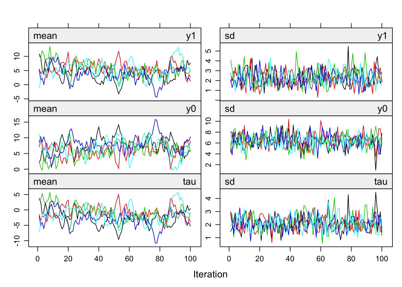
Figure 8.2: Trace lines of FCS with a \(\rho = 0.9\) and \(m = 5\).
The trace lines in Figure 8.2, produced by plot(imp), look well-behaved. Imputations of y1 and y0 hover in the same range, but imputations for y0 have more spread. Note that tau (the average over the individual causal effects) is mostly negative.
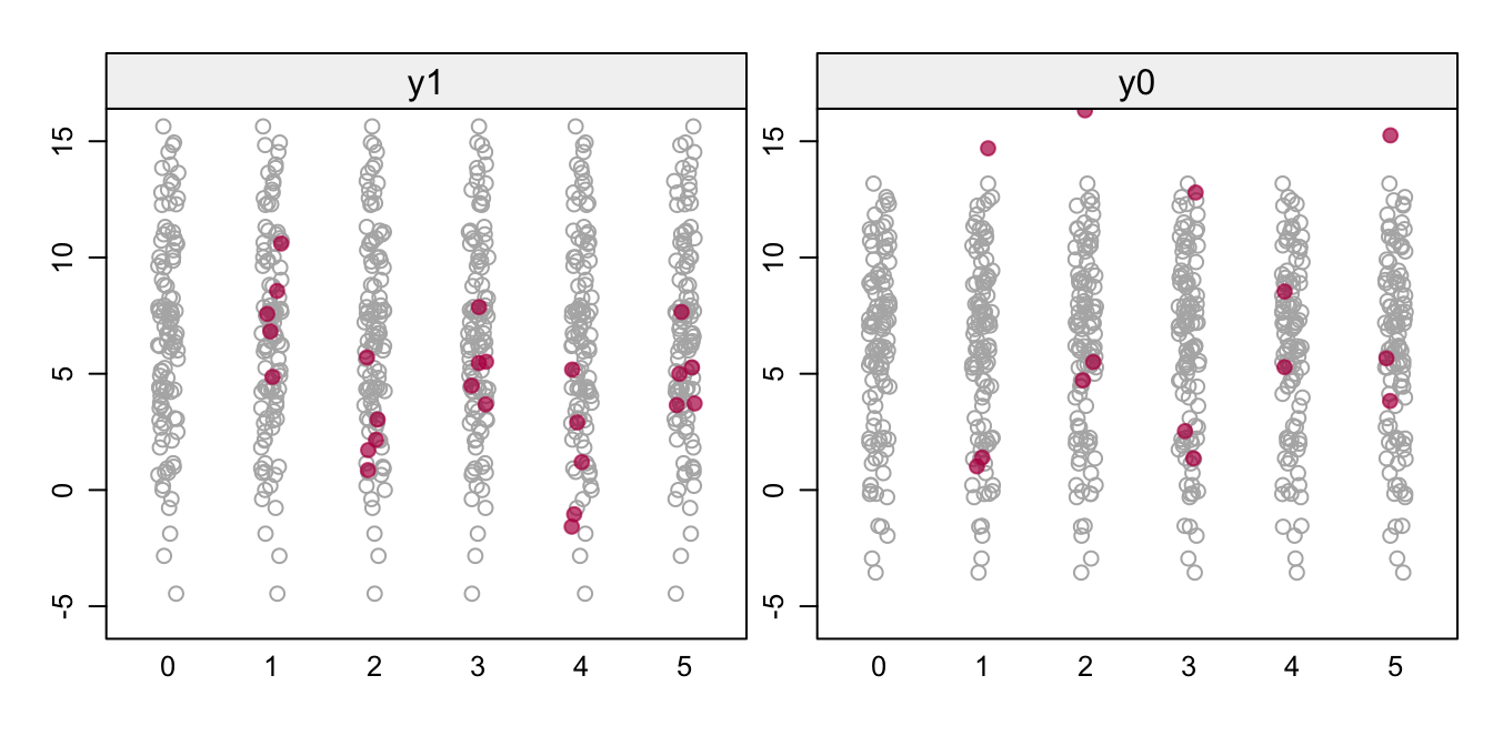
Figure 8.3: FCS with a \(\rho\) prior. Stripplots of the prior data (gray) and the imputed data (red) for the potential outcomes y1 and y0.
Figure 8.3 shows the imputed data (red) against a backdrop of the prior of 100 data points. The left-hand plot shows the imputations for the five patients who received the standard surgery, while the right-hand plot shows imputations for the three patients who received the new surgery. Although there are a few illogical negative values, most imputations are in a plausible range. The correlations between y1 and y0 vary around the expected value of 0.9:
sapply(mice::complete(imp, "all"), function(x) {
  x <- x[x$d == 1, ]; cor(x$y0, x$y1)})
1 2 3 4 5
0.952 0.976 0.960 0.953 0.840 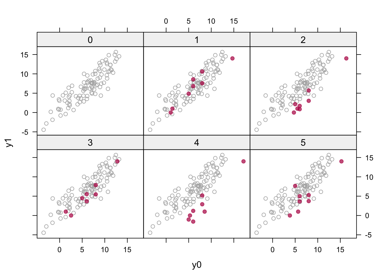
Figure 8.4: Multiple imputation (\(m = 5\)) of the potential outcomes (in red) plotted against the hypothetical prior data (in gray) with \(\rho = 0.9\).
Figure 8.4 is created as
xyplot(imp, y1 ~ y0 | as.factor(.imp), layout = c(3, 2),
       groups =  d, col = c("grey70", mdc(2)), pch = c(1, 19))
It visualizes the eight pairs of imputed potential outcomes against a backdrop of the hypothetical prior data. The imputed values are now reasonably behaved in the sense that they look like the prior data. Note that the red points may move as a whole in the horizontal or vertical directions (e.g., as in imputation 4) as the norm method draws the regression parameters from their respective posteriors to account for the sampling uncertainty of the imputation model.
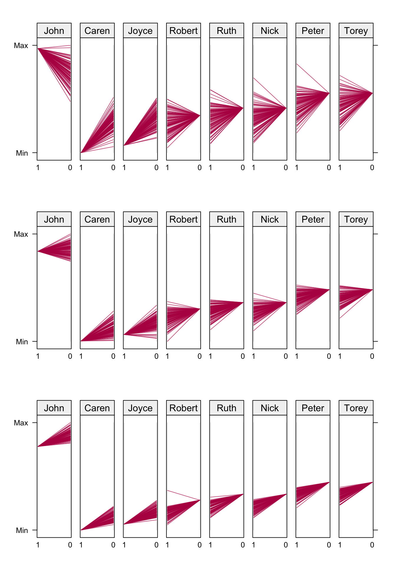
Figure 8.5: Fan plot. Observed and imputed (\(m = 100\)) outcomes under new (1) and standard (0) surgery. John, Caren and Joyce had the new surgery. The three rows correspond to \(\rho = 0.00\) (top), \(\rho = 0.90\) (middle) and \(\rho = 0.99\) (bottom). Data from Table 8.1.
Figure 8.5 displays imputations by patients for three different values of \(\rho\). Each panel contains the observed outcome for the patient, and \(m = 100\) imputed values for the missing outcome. We used \(\sigma_0^2 = \sigma_1^2 = 1\) here. John, Caren and Joyce had the new surgery, so in their panel the observed value is at the left-hand side (labeled 1), and the imputed 100 values are on the right-hand side (labeled 0). The direction is reversed for patients that had standard surgery. The values are connected, resulting in a fan-shaped image.
For \(\rho = 0\), there is substantial regression to the global mean in the imputed values. For example, John’s imputed outcomes are nearly all lower than his observed value, whereas the opposite occurs for Caren. John would benefit from the new surgery, whereas Caren would benefit from the standard treatment. Thus, for \(\rho = 0\) there is a strong tendency to pull the imputations towards the mean. The effects are heterogeneous. Convergence of this condition is very quick.
The pattern for the \(\rho = 0.99\) condition (bottom row) is different. All patients would benefit from the standard surgery, but the magnitude of the benefit is smaller than those under \(\rho = 0\). Observe that all effects, except for Caren and Joyce, go against the direction of the regression to the mean. The effects are almost identical, and the between-imputation variance is small. The solution in the middle row (\(\rho = 0.9\)) is a compromise between the two. Intuitively, this setting is perhaps the most realistic and reasonable.
8.4.3 Extensions
Imbens and Rubin (2015) observe that the inclusion of covariates does not fundamentally change the underlying method for imputing the missing outcomes. This generalizes Neyman’s method to covariates, and has the advantage that covariates can improve the imputations by providing additional information on the outcomes. A clear causal interpretation is only warranted if the covariates are not influenced by the treatment. This includes pre-treatment factors that led up to the decision to treat or not (e.g., age, disease history), pre-treatment factors that are predictive of the later outcome, such as baseline outcomes, and post-treatment factors that are not affected by treatment. Covariates that may have changed as a result of the experimental treatment should not be included in a causal model.
We may distinguish various types of covariates. A covariate can be part of the assignment mechanism, related to the potential outcomes \(Y_i(0)\) and \(Y_i(1)\), or related to \(\tau_i\). The first covariate type is often included into the imputation model in order to account for design effects, in particular to achieve comparability of the experimental units. A causal effect must be a comparison of the ordered sets \(\{Y_i(1), i \in S\}\) and \(\{Y_i(0), i \in S\}\) (Rubin 2005), which can always be satisfied once the potential outcomes have been imputed for units \(i \in S\). Hence, we have no need to stratify on design variables to achieve comparability. However, we still need to include design factors into the imputation model in order to satisfy the condition of ignorable treatment assignment. Including the second covariate type will make the imputations more precise, and so this is generally beneficial. The third covariate type directly explains heterogeneity of causal effects over the units. Because \(\tau_i\) is an entirely missing (latent) variable, it is difficult to impute \(\tau_i\) directly in mice. The method in Section 8.4.2 explains heterogeneity of \(\tau_i\) indirectly via the imputation models for \(Y_i(0)\) and \(Y_i(1)\). Any covariates of type 3 should be included on the imputation models, and their regression weights should be allowed to differ between models for \(Y_i(0)\) and \(Y_i(1)\).
Suppose we wish to obtain the average causal effect for \(n_S > 1\) units \(i \in S\). Calculate the within-replication average causal effect \(\tau_\ell\) over the units in set \(S\) as
\[ \dot\tau_\ell = \frac{1}{n_S}\sum_{i \in S} \dot\tau_{i\ell} \tag{8.12} \]
and its variance as
\[ \dot\sigma_\ell^2 = \frac{1}{n_S-1} \sum_{i \in S} (\dot\tau_{i\ell} - \dot\tau_\ell)^2 \tag{8.13} \]
and then combine the results over the replications by means of Rubin’s rules. We can use the same principles for categorical outcomes. Mortality is a widely used outcome, and can be imputed by logistic regression. The ICE can then takes on one of four possible values: (alive, alive), (alive, dead), (dead, alive) and (dead, dead). An still open question is how the dependency between the potential outcomes is best specified.
We may add a potential outcome for every additional treatment, so extension to three or more experimental conditions does not present new conceptual issues. However the imputation problem becomes more difficult. With four treatments, 75 percent of each outcome will need to be imputed, and the number of outcomes to impute will double. There are practical limits to what can be done, but I have done analyses with seven treatment arms. Careful monitoring of convergence is needed, as well as a reasonably size dataset in each experimental group.
After imputation, the individual causal effect estimates can be analyzed for patterns that explain the heterogeneity. The simplest approach takes \(\hat\tau_i\) as the outcome for a regression at the unit level, and ignores the often substantial variation around \(\hat\tau_i\). This is primarily useful for exploratory analysis. Alternatively, we may utilize the full multiple imputation cycle, so perform the regression on \(\dot\tau_{i\ell}\) within each imputed dataset, and then pool the results by Rubin’s rules.