11.2 SE Fireworks Disaster Study
On May 13, 2000, a catastrophic fireworks explosion occurred at SE Fireworks in Enschede, the Netherlands. The explosion killed 23 people and injured about 950. Around 500 houses were destroyed, leaving 1250 people homeless. Ten thousand residents were evacuated.
The disaster marked the starting point of a major operation to recover from the consequences of the explosion. Over the years, the neighborhood has been redesigned and rebuilt. Right after the disaster, the evacuees were relocated to improvised housing. Those in need received urgent medical care. A considerable number of residents showed signed of post-traumatic stress disorder (PTSD). This disorder is associated with flashback memories, avoidance of behaviors, places, or people that might lead to distressing memories, sleeping disorders and emotional numbing. When these symptoms persist and disrupt normal daily functioning, professional treatment is indicated.
Amidst the turmoil in the aftermath, Mediant, the disaster health after-care center, embedded a randomized controlled trial comparing two treatments for anxiety-related disorders: eye movement desensitization and reprocessing (EMDR) (Shapiro 2001) and cognitive behavioral therapy (CBT) (Stallard 2006). CBT is the standard therapy. The data collection started within one year of the explosion, and lasted until the year 2004 (De Roos et al. 2011). The study included \(n\) = 52 children 4-18 years, as well as their parents. Children were randomized to EMDR or CBT by a flip of the coin. Each group contained 26 children.
The children received up to four individual sessions over a 4-8 week period, along with up to four parent sessions. Blind assessment took place pre-treatment (T1) and post-treatment (T2) and at 3 months follow-up (T3). The primary outcomes were the UCLA PTSD Reaction Index (PTSD-RI) (Steinberg et al. 2004), the Child Report of Post-traumatic Symptoms (CROPS) and the Parent Report of Post-traumatic Symptoms (PROPS) (Greenwald and Rubin 1999). Treatment was stopped if children were asymptomatic according to participant and parent verbal report (both conditions), or if there was no remaining distress associated with the trauma memory, as indicated by a self-reported Subjective Units of Disturbance Scale (SUDS) of 0 (EMDR condition only).
The objective of the study was to answer the following questions:
Is one of these treatments more effective in reducing PTSD symptoms at T2 and T3?
Does the number of sessions needed to produce the therapeutic effect differ between the treatments?
11.2.1 Intention to treat
| id | trt | pp | \(Y^c_1\) | \(Y^c_2\) | \(Y^c_3\) | \(Y^p_1\) | \(Y^p_2\) | \(Y^p_3\) |
|---|---|---|---|---|---|---|---|---|
| 1 | E | Y | - | - | - | 36 | 35 | 38 |
| 2 | C | N | 45 | - | - | - | - | - |
| 3 | E | N | - | - | - | 13 | 19 | 13 |
| 4 | C | Y | - | - | - | 33 | 27 | 20 |
| 5 | E | Y | 26 | 6 | 4 | 27 | 16 | 11 |
| 6 | C | Y | 8 | 1 | 2 | 32 | 15 | 13 |
| 7 | C | Y | 41 | 26 | 31 | - | 39 | 39 |
| 8 | C | N | - | - | - | 24 | 13 | 35 |
| 10 | C | Y | 35 | 27 | 14 | 48 | 23 | - |
| 12 | C | Y | 28 | 15 | 13 | 45 | 33 | 36 |
| 13 | E | Y | - | - | - | 26 | 17 | 14 |
| 14 | C | Y | 33 | 8 | 9 | 37 | 7 | 3 |
| 15 | E | Y | 43 | - | 7 | 25 | 27 | 1 |
| 16 | C | Y | 50 | 8 | 35 | 39 | 21 | 34 |
| 17 | C | Y | 31 | 21 | 10 | 32 | 21 | 19 |
| 18 | E | Y | 30 | 17 | 16 | 47 | 28 | 34 |
| 19 | E | Y | 29 | 6 | 5 | 20 | 14 | 11 |
| 20 | E | Y | 47 | 14 | 22 | 44 | 21 | 25 |
| 21 | C | Y | 39 | 12 | 12 | 39 | 5 | 19 |
| 23 | C | Y | 14 | 12 | 5 | 29 | 9 | 4 |
| 24 | E | N | 27 | - | - | - | - | - |
| 25 | E | Y | 6 | 10 | 5 | 25 | 16 | 16 |
| 28 | C | Y | - | 2 | 6 | 36 | 17 | 23 |
| 29 | E | Y | 23 | 23 | 28 | 23 | 25 | 13 |
| 30 | E | Y | - | - | - | 20 | 23 | 12 |
| 31 | C | N | 15 | 24 | 26 | 33 | 36 | 38 |
| 32 | E | N | 28 | 17 | 8 | 40 | 42 | 33 |
| 33 | E | N | - | - | - | 38 | 22 | 25 |
| 34 | E | N | - | - | - | 17 | - | - |
| 35 | E | Y | 50 | 20 | - | 19 | 1 | 5 |
| 37 | C | N | 30 | - | 26 | 59 | - | 28 |
| 38 | C | Y | - | - | - | 35 | 24 | 27 |
| 39 | E | N | - | - | - | - | - | - |
| 40 | E | Y | 25 | 5 | 2 | 42 | 13 | 11 |
| 41 | E | Y | 36 | 11 | 9 | 30 | 2 | 1 |
| 43 | E | N | 17 | - | - | - | - | - |
| 44 | E | N | 27 | - | - | 40 | - | - |
| 45 | C | Y | 31 | 12 | 29 | 34 | 28 | 29 |
| 46 | C | Y | - | - | - | 44 | 35 | 25 |
| 47 | C | Y | - | - | - | 30 | 18 | 14 |
| 48 | E | Y | 25 | 18 | - | 18 | 17 | 2 |
| 49 | C | N | 24 | 23 | 16 | 44 | 29 | 34 |
| 50 | E | Y | 31 | 13 | 9 | 34 | 18 | 13 |
| 51 | C | Y | - | - | - | 52 | 13 | 13 |
| 52 | C | Y | 30 | 35 | 28 | - | 44 | 50 |
| 53 | C | Y | 19 | 33 | 21 | 36 | 21 | 21 |
| 54 | C | N | 43 | - | - | 48 | - | - |
| 55 | E | Y | 64 | 42 | 35 | 44 | 31 | 16 |
| 56 | C | Y | - | - | - | 37 | 6 | 9 |
| 57 | C | Y | 31 | 12 | - | 32 | 26 | - |
| 58 | E | Y | - | - | - | 49 | 28 | 25 |
| 59 | E | Y | 39 | 7 | - | 39 | 7 | - |
Table 11.1 contains the outcome data of all subjects. The columns labeled \(Y^c_t\) contain the child data, and the columns labeled \(Y^p_t\) contain the parent data at time \(t\) = (1, 2, 3). Children under the age of 6 years did not fill in the child form, so their scores are missing.
Of the 52 initial participants 14 children (8 EMDR, 6 CBT) did not follow the protocol. The majority (11) of this group did not receive the therapy, but still provided outcome measurements. The three others received therapy, but failed to provide outcome measures. The combined group is labeled as “drop-out,” while the other group is called the “completers” or “per-protocol” group. Figure 11.1 shows the missing data patterns for both groups.
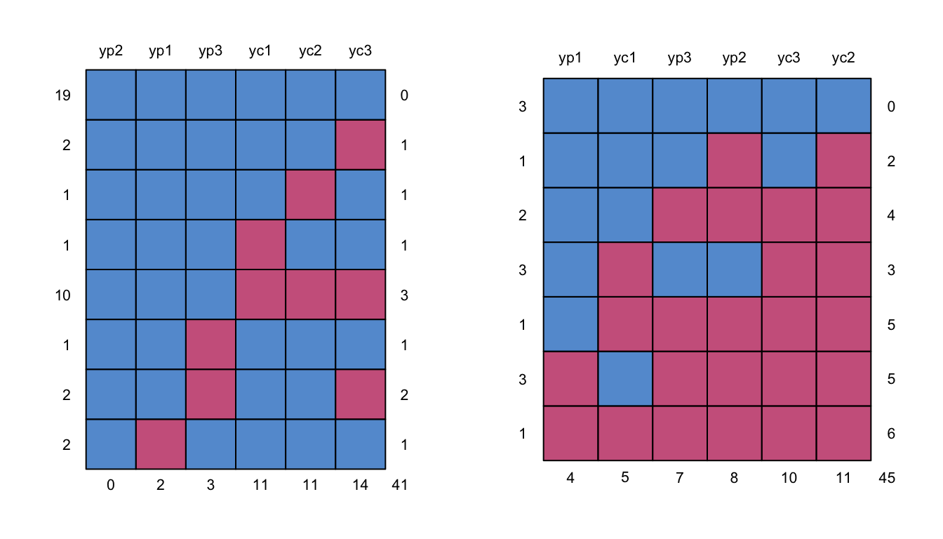
Figure 11.1: Missing data patterns for the “per-protocol” group (left) and the “drop-out” group (right).
The main reason given for dropping out was that the parents were overburdened (8). Other reasons for dropping out were: refusing to talk (1), language problems (1) and a new trauma rising to the forefront (2). One adolescent refused treatment from a therapist not belonging to his own culture (1). One child showed spontaneous recovery before treatment started (1).
Comparison between the 14 drop-outs and the 38 completers regarding presentation at time of initial assessment yielded no significant differences in any of the demographic characteristics or number of traumatic experiences. On the symptom scales, only the mean score of the PROPS was marginally significantly higher for the drop-out group than for the treatment completers (\(t\) = 2.09, \(\mathrm{df}\) = 48, \(p\) = .04).
Though these preliminary analyses are comforting, the best way to analyze the data is to the compare participants in the groups to which they were randomized, regardless of whether they received or adhered to the allocated intervention. Formal statistical testing requires random assignment to groups. The intention to treat (ITT) principle is widely recommended as the preferred approach to the analysis of clinical trials. DeMets, Cook, and Roecker (2007) and White et al. (2011) provide balanced discussions of pros and cons of ITT.
11.2.2 Imputation model
The major problem of the ITT principle is that some of the data that are needed are missing. Multiple imputation is a natural way to solve this problem, and thus to enable ITT analyses.
A difficulty in setting up the imputation model in the SE Fireworks Disaster Study is the large number of outcome variables relative to the number of cases. Even though the analysis of the data in Table 11.1 is already challenging, the real dataset is more complex than this. There are six additional outcome variables (e.g., the Child Behavior Checklist, or CBCL), each measured over time and similarly structured as in Table 11.1. In addition, some of the outcome measures are to be analyzed on both the subscale level and the total score level. For example, the PTSD-RI has three subscales (intrusiveness/numbing/avoidance, fear/anxiety, and disturbances in sleep and concentration and two additional summary measures (full PTSD and partial PTSD). All in all, there were 65 variables in data to be analyzed. Of these, 49 variables were incomplete. The total number of cases was 52, so in order to avoid grossly overdetermined models, the predictors of the imputation model should be selected very carefully.
A first strategy for predictor reduction was to preserve all deterministic relations columns in the incomplete data. This was done by passive imputation. For example, let \(Y^p_{a,1}\), \(Y^p_{b,1}\) and \(Y^p_{c,1}\) represent the scores on three subscales of the PTSD parent form administered at T1. Each of these is imputed individually. The total variable \(Y^p_1\) is then imputed by mice in a deterministic way as the sum score.
A second strategy to reduce the number of predictors was to leave out other outcomes, measured at other time points. To illustrate this, a subset of the predictor matrix for imputing \(Y^p_{a,1}\), \(Y^p_{b,1}\) and \(Y^p_{c,1}\) is:
vars <-c("ypa1", "ypb1", "ypc1",
         "ypa2", "ypb2", "ypc2",
         "ypa3", "ypb3", "ypc3")
fdd.pred[vars[1:3], vars]
ypa1 ypb1 ypc1 ypa2 ypb2 ypc2 ypa3 ypb3 ypc3
ypa1 0 1 1 1 0 0 1 0 0
ypb1 1 0 1 0 1 0 0 1 0
ypc1 1 1 0 0 0 1 0 0 1The conditional distribution \(P(Y^p_{a,1}|Y^p_{b,1}, Y^p_{c,1}, Y^p_{a,2}, Y^p_{a,3})\) leaves out the cross-lagged predictors \(Y^p_{b,2}\), \(Y^p_{c,2}\), \(Y^p_{b,3}\) and \(Y^p_{c,3}\). The assumption is the cross-lagged predictors are represented by through their non-cross-lagged predictors. Applying this idea consistently throughout the entire 65 \(\times\) 65 predictor matrix brings vast reductions of the number of predictors. The largest number of predictors for any incomplete variable was 23, which still leaves degrees of freedom for residual variation.
Specifying a 65 \(\times\) 65 predictor matrix by syntax in R is tedious and prone to error. I copied the variable names to Microsoft Excel, defined a square matrix of small cells containing zeroes, and used the menu option Conditional formatting... to define a cell color if the cell contains a “1.” The option Freeze Panes was helpful for keeping variable names visible at all times. After filling in the matrix with the appropriate patterns of ones, I exported it to R to be used as argument to the mice() function. Excel is convenient for setting up large, patterned imputation models.
The imputations were generated as
meth <- make.method(fdd)
meth["yc1"] <- "~I(yca1 + ycb1 + ycc1)"
meth["yc2"] <- "~I(yca2 + ycb2 + ycc2)"
meth["yc3"] <- "~I(yca3 + ycb3 + ycc3)"
meth["yp1"] <- "~I(ypa1 + ypb1 + ypc1)"
meth["yp2"] <- "~I(ypa2 + ypb2 + ypc2)"
meth["yp3"] <- "~I(ypa3 + ypb3 + ypc3)"
imp <- mice(fdd, pred = fdd.pred, meth = meth, maxit = 20,
            seed = 54434, print = FALSE)
11.2.3 Inspecting imputations
For plotting purposes we need to convert the imputed data into long form. In R this can be done as follows:
lowi <- mice::complete(imp, "long", inc=TRUE)
lowi <- data.frame(lowi,cbcl2=NA, cbin2=NA,cbex2=NA)
lolo <- reshape(lowi, idvar = 'id',
                varying = 11:ncol(lowi),
                direction = "long",
                new.row.names = 1:(nrow(lowi)*3),
                sep="")
lolo <- lolo[order(lolo$.imp, lolo$id, lolo$time),]
row.names(lolo) <- 1:nrow(lolo)
This code executes two wide-to-long transformations in succession. The data are imputed in wide format. The call to complete() writes the \(m\) + 1 imputed stacked datasets to lowi, which stands for “long-wide.” The data.frame() statement appends three columns to the data with missing CBCL scores, since the CBCL was not administered at time point 2. The reshape() statement interprets everything from column 11 onward as time-varying variables. As long as the variables are labeled consistently, reshape() will be smart enough to identify groups of columns that belong together, and stack them in the double-long format lolo. Finally, the result is sorted such that the original data with lolo$.imp==0 are stored as the first block.
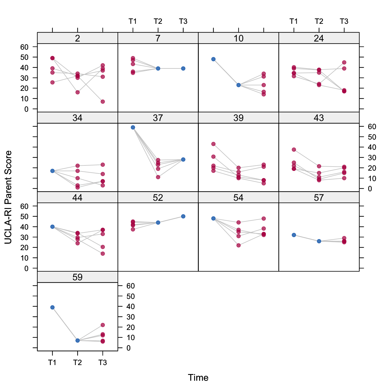
Figure 11.2: Plot of the multiply imputed data of the 13 subjects with one or more missing values on PTSD-RI parent form.
Figure 11.2 plots the profiles from 13 subjects with a missing score on \(Y^p_1\), \(Y^p_2\) or \(Y^p_3\) in Table 11.1. Some profiles are partially imputed. Examples are subjects 7 (missing T1) and 37 (missing T2). Other profiles are missing entirely, and are thus completely imputed. Examples are subjects 2 and 43. Similar plots can be made for other outcomes. In general, the imputed profiles look similar to the completely observed profiles (not shown).
11.2.4 Complete-data model
In the absence of missing data, we would have liked to perform a classical repeated measures MANOVA as in Potthoff and Roy (1964). This method construct derived variables that represent time as polynomial contrasts that can be tested. An appealing feature of the method is that the covariances among the repeated measures can take any form.
Let \(y_{ikt}\) denote the measurement of individual \(i\) (\(i=1,\dots,n_k\)) in group \(k\) (CBT or EMDR) at time point \(t\) (\(t=1,\dots,n_t\)). In the SE Fireworks Disaster Study data, we have \(n_k=26\) and \(n_t=3\). All subjects have been measures at the same time points. The model represents the time trend in each group by a linear and quadratic trend as
\[ y_{ikt}=\beta_{k0}+t \beta_{k1} + t^2 \beta_{k2} + e_{ikt} \tag{11.1} \]
where the subject residual \(e_i\) has an arbitrary covariance 3 \(\times\) 3 matrix \(\Sigma\) that is common to both groups. This model has six \(\beta\) parameters, three for each treatment group. To answer the first research question, we would be interested in testing the null hypotheses \(\beta_{11}=\beta_{21}\) and \(\beta_{12}=\beta_{22}\), i.e., whether the linear and quadratic trends are different between the treatment groups.
Potthoff and Roy (1964) showed how this model can be transformed into the usual MANOVA model and be fitted by standard software. Suppose that the repeated measures are collected in variables Y1, Y2 and Y3. In SPSS we can use the GLM command to test for the hypothesis of linear and quadratic time trends, and for the hypothesis that these trends are different between CBT and EMDR groups. Though application of the method is straightforward for complete data, it cannot be used directly for the SE Fireworks Disaster Study, because of the missing data.
The mids object created by mice() can be exported as a multiply imputed dataset to SPSS by means of the mids2spss() function. If the data came originally from SPSS it is also possible to merge the imputed data with the original data by means of the UPDATE command. SPSS will recognize an imported multiply imputed dataset, and execute the analysis \(m\) times in parallel. It can also provide the pooled statistics. Note that pooling requires a license to the Missing Values module.
Unfortunately, in SPSS 18.0 pooling is not implemented for GLM. As a solution, I stored the results by means of the OMS command in SPSS and shipped the output back to R for further analysis. I then applied a yet unpublished procedure for pooling \(F\)-tests to the datasets stored by the OMS command. In this way, pooling procedures that are not built into SPSS can be done with mice.
Of course, I could have saved myself the trouble of exporting the imputed data to SPSS and performed all analyses in R. That would, however, lock out the investigator from her own data. With the new pooling facilities investigators can now do their own data analysis on multiply imputed data. Some re-exporting is therefore worthwhile.
An alternative could have been to create the multiply imputed datasets within SPSS. This option was not possible for these data because the MULTIPLE IMPUTATION command in SPSS does not support predictor selection and passive imputation. With a bit of conversion between software packages, it is possible to have best of both worlds.
11.2.5 Results from the complete-data model
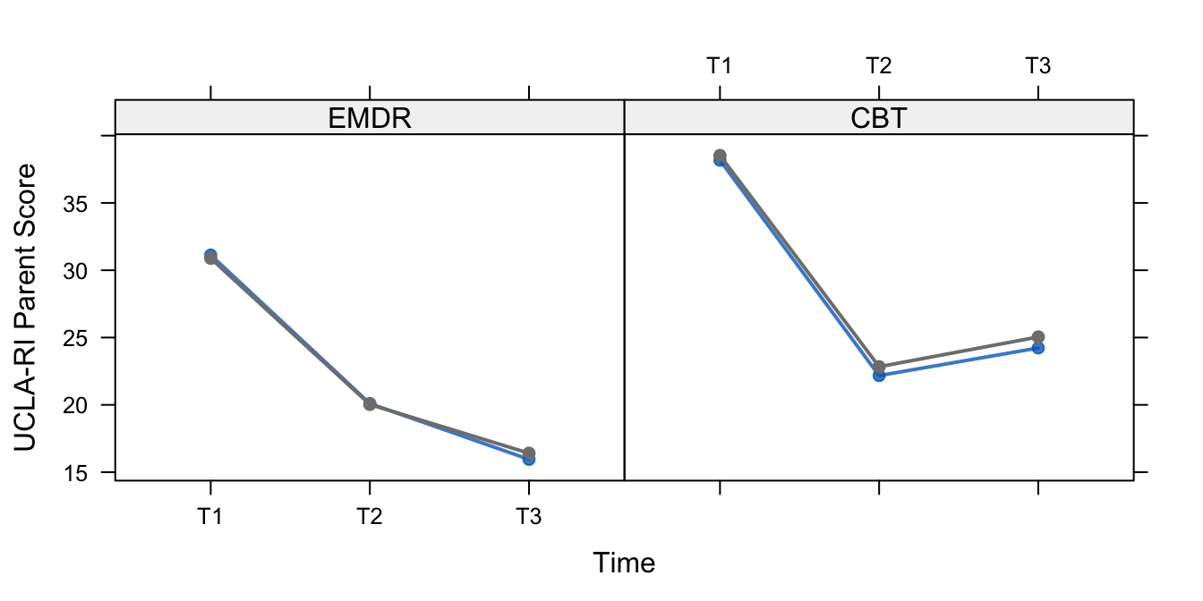
Figure 11.3: Mean levels of PTSD-RI parent form for the completely observed profiles (blue) and all profiles (black) in the EMDR and CBT groups.
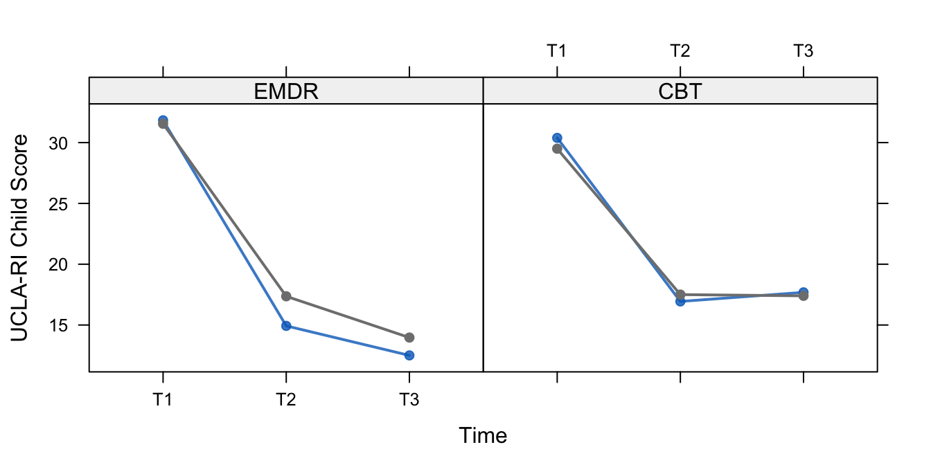
Figure 11.4: Mean levels of PTSD-RI Child Form for the completely observed profiles (blue) and all profiles (black) in the EMDR and CBT groups.
Figures 11.3 and 11.4 show the development of the mean level of PTSD complaint according to the PTSD-RI. All curves display a strong downward trend between start of treatment (T1) and end of treatment (T2), which is presumably caused by the EMDR and CBT therapies. The shape between end of treatment (T2) and follow-up (T3) differs somewhat for the group, suggesting that EMDR has better long-term effects, but this difference was not statistically significant. Also note that the complete-case analysis and the analysis based on ITT are in close agreement with each other here.
We will not go into details here to answer the second research question as stated on page . It is of interest to note that EMDR needed fewer sessions to achieve its effect. The original publication (De Roos et al. 2011) contains the details.