3.3 Imputation under non-normal distributions

3.3.1 Overview

The imputation methods discussed in Section 3.2 produce imputations drawn from a normal distribution. In practice the data could be skewed, long tailed, non-negative, bimodal or rounded, to name some deviations from normality. This creates an obvious mismatch between observed and imputed data which could adversely affect the estimates of interest.

The effect of non-normality is generally small for measures that rely on the center of the distribution, like means or regression weights, but it could be substantial for estimates like a variance or a percentile. In general, normal imputations appear to be robust against violations of normality. Demirtas, Freels, and Yucel (2008) found that flatness of the density, heavy tails, non-zero peakedness, skewness and multimodality do not appear to hamper the good performance of multiple imputation for the mean structure in samples \(n>400\), even for high percentages (75%) of missing data in one variable. The variance parameter is more critical though, and could be off-target in smaller samples.

One approach is to transform the data toward normality before imputation, and back-transform them after imputation. A beneficial side effect of transformation is that the relation between \(x\) and \(y\) may become closer to a linear relation. Sometimes applying a simple function to the data, like the logarithmic or inverse transform, is all that is needed. More generally, the transformation could be made to depend on known covariates like age and sex, for example as done in the LMS model (Cole and Green 1992) or the GAMLSS model (Rigby and Stasinopoulos 2005).

Von Hippel (2013) warns that application of tricks to make the distribution of skewed variables closer to normality (e.g., censoring, truncation, transformation) may make matters worse. Censoring (rounding a disallowed value to the nearest allowed value) and truncation (redrawing a disallowed value until it is within the allowed range) can change both the mean and variability in the data. Transformations may fail to achieve near-normality, and even if that succeeds, bivariate relations may be affected when imputed by a method that assumes normality. The examples of Von Hippel are somewhat extreme, but they do highlight the point that simple fixes to achieve normality are limited by what they can do.

There are two possible strategies to progress. The first is to use predictive mean matching. Section 3.4 will describe this approach in more detail. The other strategy is to model the non-normal data, and to directly draw imputations from those models. Liu (1995) proposed methods for drawing imputations under the \(t\)-distribution instead of the normal. He and Raghunathan (2006) created imputations by drawing from Tukey’s \(gh\)-distribution, which can take many shapes. Demirtas and Hedeker (2008a) investigated the behavior of methods for drawing imputation from the Beta and Weibull distributions. Likewise, Demirtas and Hedeker (2008b) took draws from Fleishman polynomials, which allows for combinations of left and right skewness with platykurtic and leptokurtic distributions.

The GAMLSS method (Rigby and Stasinopoulos 2005; Stasinopoulos et al. 2017) extends both the generalized linear model and the generalized additive model. A unique feature of GAMLSS is its ability to specify a (possibly nonlinear) model for each of the parameters of the distribution, thus giving rise to an extremely flexible toolbox that can be used to model almost any distribution. The gamlss package contains over 60 built-in distributions. Each distribution comes with a function to draw random variates, so once the gamlss model is fitted, it can also be used to draw imputations. The first edition of this book showed how to construct a new univariate imputation function that mice could call. This is not needed any more. De Jong (2012) and De Jong, Van Buuren, and Spiess (2016) developed a series of imputation methods based on GAMLSS, so it is now easy to perform multiple imputation under variety of distributions. The ImputeRobust package (Salfran and Spiess 2017), implements various mice methods for continuous data: gamlss (normal), gamlssJSU (Johnson’s SU), gamlssTF (\(t\)-distribution) and gamlssGA (gamma distribution). The following section demonstrates the use of the package.

3.3.2 Imputation from the \(t\)-distribution

We illustrate imputation from the \(t\)-distribution. The \(t\)-distribution is favored for more robust statistical modeling in a variety of settings (Lange, Little, and Taylor 1989). Van Buuren and Fredriks (2001) observed unexplained kurtosis in the distribution of head circumference in children. Rigby and Stasinopoulos (2006) fitted a \(t\)-distribution to these data, and observed a substantial improvement of the fit.

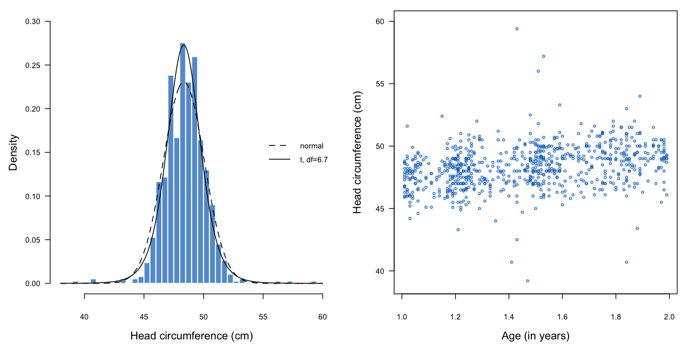
Figure 3.4: Measured head circumference of 755 Dutch boys aged 1–2 years (Fredriks, Van Buuren, Burgmeijer, et al. 2000).

Figure 3.4 plots the data for Dutch boys aged 1–2 years. Due to the presence of several outliers, the \(t\)-distribution with 6.7 degrees of freedom fits the data substantially better than the normal distribution (Akaike Information Criterion (AIC): 2974.5 (normal model) versus 2904.3 (\(t\)-distribution). If the outliers are genuine data, then the \(t\)-distribution should provide imputations that are more realistic than the normal.

We create a synthetic dataset by imputing head circumference of the same 755 boys. Imputation is easily done with the following steps: append the data with a duplicate, create missing data in hc and run mice() calling the gamlssTF method as follows:

library("ImputeRobust")
library("gamlss")
data(db)
data <- subset(db, age > 1 & age < 2, c("age", "head"))
names(data) <- c("age", "hc")
synthetic <- rep(c(FALSE, TRUE), each = nrow(data))
data2 <- rbind(data, data)
row.names(data2) <- 1:nrow(data2)
data2[synthetic, "hc"] <- NA
imp <- mice(data2, m = 1, meth = "gamlssTF", seed = 88009,
            print = FALSE)
syn <- subset(mice::complete(imp), synthetic)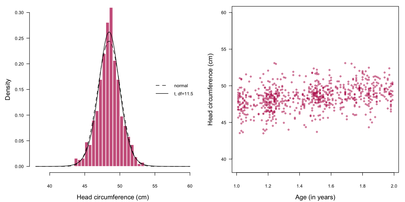

Figure 3.5: Fully synthetic data of head circumference of 755 Dutch boys aged 1–2 years using a \(t\)-distribution.

Figure 3.5 is the equivalent of Figure 3.4, but now calculated from the synthetic data. Both configurations are similar. As expected, some outliers also occur in the imputed data, but these are a little less extreme than in the observed data due to the smoothing by the \(t\)-distribution. The estimated degrees of freedom varies over replications, and appears to be somewhat larger than the value of 6.7 estimated from the observed data. For this replication, it is larger (11.5). The distribution of the imputed data is better behaved compared to the observed data. The typical rounding patterns seen in the real measurements are not present in the imputed data. Though these are small differences, they may be of relevance in particular analyses.