1.4 Multiple imputation in a nutshell
1.4.1 Procedure
Multiple imputation creates \(m>1\) complete datasets. Each of these datasets is analyzed by standard analysis software. The \(m\) results are pooled into a final point estimate plus standard error by pooling rules (“Rubin’s rules”). Figure 1.6 illustrates the three main steps in multiple imputation: imputation, analysis and pooling.
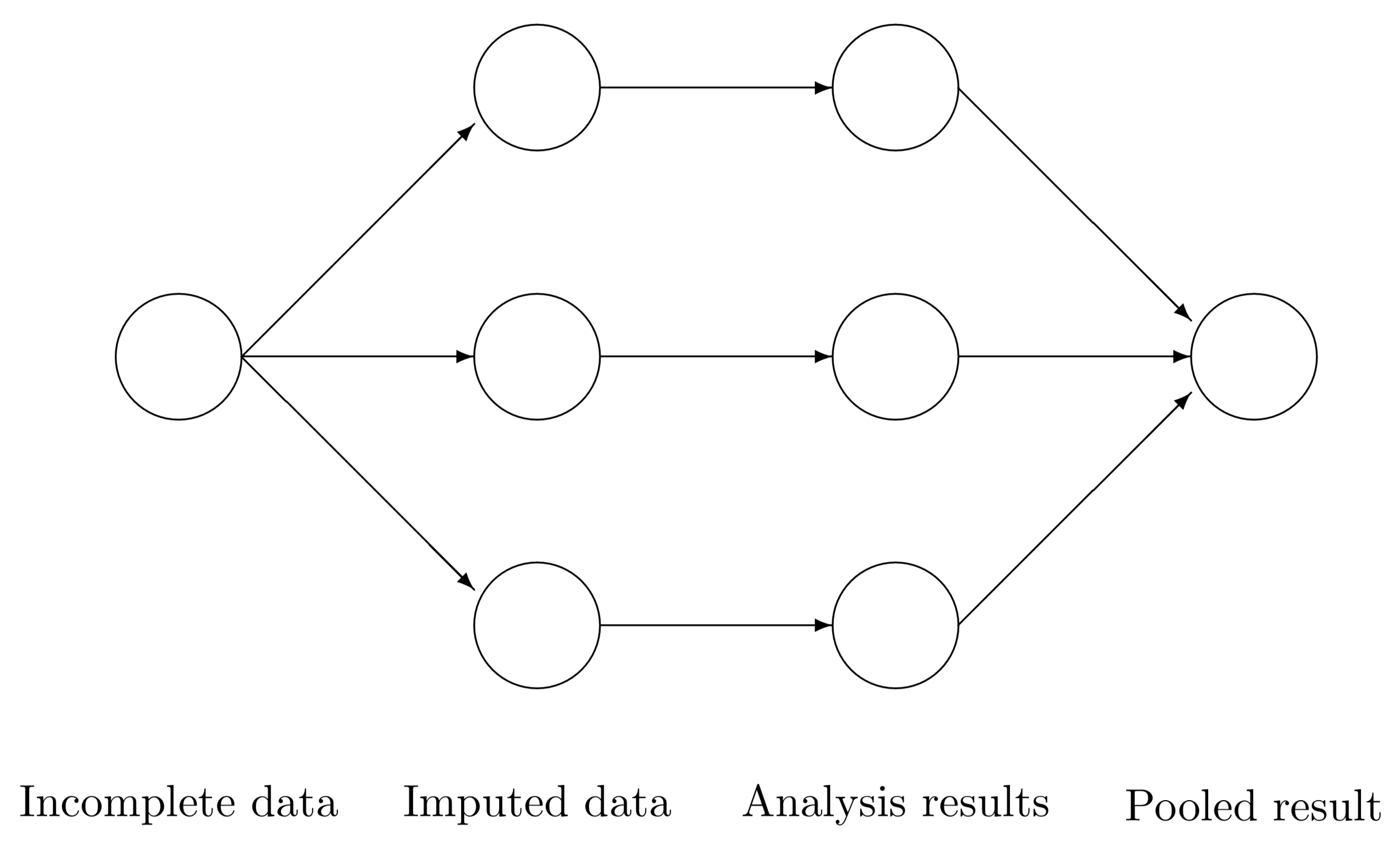
Figure 1.6: Scheme of main steps in multiple imputation.
The analysis starts with observed, incomplete data. Multiple imputation creates several complete versions of the data by replacing the missing values by plausible data values. These plausible values are drawn from a distribution specifically modeled for each missing entry. Figure 1.6 portrays \(m=3\) imputed datasets. In practice, \(m\) is often taken larger (cf. Section 2.8). The number \(m=3\) is taken here just to make the point that the technique creates multiple versions of the imputed data. The three imputed datasets are identical for the observed data entries, but differ in the imputed values. The magnitude of these difference reflects our uncertainty about what value to impute.
The second step is to estimate the parameters of interest from each imputed dataset. This is typically done by applying the analytic method that we would have used had the data been complete. The results will differ because their input data differ. It is important to realize that these differences are caused only because of the uncertainty about what value to impute.
The last step is to pool the \(m\) parameter estimates into one estimate, and to estimate its variance. The variance combines the conventional sampling variance (within-imputation variance) and the extra variance caused by the missing data extra variance caused by the missing data (between-imputation variance). Under the appropriate conditions, the pooled estimates are unbiased and have the correct statistical properties.
1.4.2 Reasons to use multiple imputation
Multiple imputation (Rubin 1987b; Rubin 1996) solves the problem of “too small” standard errors in Table 1.1. Multiple imputation is unique in the sense that it provides a mechanism for dealing with the inherent uncertainty of the imputations themselves.
Our level of confidence in a particular imputed value is expressed as the variation across the \(m\) completed datasets. For example, in a disability survey, suppose that the respondent answered the item whether he could walk, but did not provide an answer to the item whether he could get up from a chair. If the person can walk, then it is highly likely that the person will also be able to get up from the chair. Thus, for persons who can walk, we can draw a “yes” for missing “getting up from a chair” with a high probability, say 0.99, and use the drawn value as the imputed value. In the extreme, if we are really certain, we always impute the same value for that person. In general however, we are less confident about the true value. Suppose that, in a growth study, height is missing for a subject. If we only know that this person is a woman, this provides some information about likely values, but not so much. So the range of plausible values from which we draw is much larger here. The imputations for this woman will thus vary a lot over the different datasets. Multiple imputation is able to deal with both high-confidence and low-confidence situations equally well.
Another reason to use multiple imputation is that it separates the solution of the missing data problem from the solution of the complete-data problem. The missing-data problem is solved first, the complete-data problem next. Though these phases are not completely independent, the answer to the scientifically interesting question is not obscured anymore by the missing data. The ability to separate the two phases simplifies statistical modeling, and hence contributes to a better insight into the phenomenon of scientific study.
1.4.3 Example of multiple imputation
Continuing with the airquality dataset, it is straightforward to apply multiple imputation. The following code imputes the missing data twenty times, fits a linear regression model to predict Ozone in each of the imputed datasets, pools the twenty sets of estimated parameters, and calculates the Wald statistics for testing significance of the weights.
imp <- mice(airquality, seed = 1, m = 20, print = FALSE)
fit <- with(imp, lm(Ozone ~ Wind + Temp + Solar.R))
summary(pool(fit))
estimate std.error statistic df p.value
(Intercept) -62.7055 21.1973 -2.96 106.3 0.003755025718
Wind -3.0839 0.6281 -4.91 91.7 0.000003024665
Temp 1.5988 0.2311 6.92 115.4 0.000000000271
Solar.R 0.0573 0.0217 2.64 112.8 0.009489765888There is much more to say about each of these steps, but it shows that multiple imputation need not be a daunting task. Assuming we have set options(na.action = na.omit), fitting the same model to the complete cases can be done by
fit <- lm(Ozone ~ Wind + Temp + Solar.R, data = airquality)
coef(summary(fit))
Estimate Std. Error t value Pr(>|t|)
(Intercept) -64.3421 23.0547 -2.79 0.00622663809
Wind -3.3336 0.6544 -5.09 0.00000151593
Temp 1.6521 0.2535 6.52 0.00000000242
Solar.R 0.0598 0.0232 2.58 0.01123663550The solutions are nearly identical here, which is due to the fact that most missing values occur in the outcome variable. The standard errors of the multiple imputation solution are slightly smaller than in the complete-case analysis. Multiple imputation is often more efficient than complete-case analysis. Depending on the data and the model at hand, the differences can be dramatic.
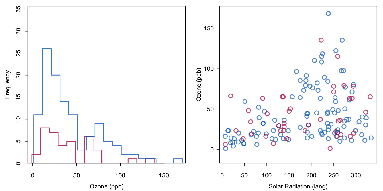
Figure 1.7: Multiple imputation of Ozone. Plotted are the imputed values from the first imputation.
Figure 1.7 shows the distribution and scattergram for the observed and imputed data combined. The imputations are taken from the first completed dataset. The blue and red distributions are quite similar. Problems with the negative values as in Figure 1.4 are now gone since the imputation method used observed data as donors to fill the missing data. Section 3.4 describes the method in detail. Note that the red points respect the heteroscedastic nature of the relation between Ozone and Solar.R. All in all, the red points look as if they could have been measured if they had not been missing. The reader can easily recalculate the solution and inspect these plots for the other imputations.
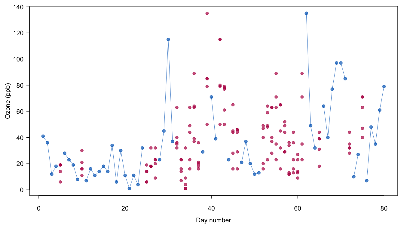
Figure 1.8: Multiple imputation of Ozone. Plotted are the observed values (in blue) and the multiply imputed values (in red).
Figure 1.8 plots the completed Ozone data. The imputed data of all five imputations are plotted for the days with missing Ozone scores. In order to avoid clutter, the lines that connect the dots are not drawn for the imputed values. Note that the pattern of imputed values varies substantially over the days. At the beginning of the series, the values are low and the spread is small, in particular for the cold and windy days 25–27. The small spread for days 25–27 indicates that the model is quite sure of these values. High imputed values are found around the hot and sunny days 35–42, whereas the imputations during the moderate days 52–61 are consistently in the moderate range. Note how the available information helps determine sensible imputed values that respect the relations between wind, temperature, sunshine and ozone.
One final point. The airquality data is a time series of 153 days. It is well known that the standard error of the ordinary least squares (OLS) estimate is inefficient (too large) if the residuals have positive serial correlation (Harvey 1981). The first three autocorrelations of the Ozone are indeed large: 0.48, 0.31 and 0.29. The residual autocorrelations are however small and within the confidence interval: 0.13, \(-0.02\) and 0.04. The inefficiency of OLS is thus negligible here.