4.1 Missing data pattern

4.1.1 Overview

Let the data be represented by the \(n \times p\) matrix \(Y\). In the presence of missing data \(Y\) is partially observed. Notation \(Y_j\) is the \(j^\mathrm{th}\) column in \(Y\), and \(Y_{-j}\) indicates the complement of \(Y_j\), that is, all columns in \(Y\) except \(Y_j\). The missing data pattern of \(Y\) is the \(n \times p\) binary response matrix \(R\), as defined in Section 2.2.3.

For both theoretical and practical reasons, it is useful to distinguish various types of missing data patterns:

1. Univariate and multivariate. A missing data pattern is said to be univariate if there is only one variable with missing data.

2. Monotone and non-monotone (or general). A missing data pattern is said to be monotone if the variables \(Y_j\) can be ordered such that if \(Y_j\) is missing then all variables \(Y_k\) with \(k>j\) are also missing. This occurs, for example, in longitudinal studies with drop-out. If the pattern is not monotone, it is called non-monotone or general.

3. Connected and unconnected. A missing data pattern is said to be connected if any observed data point can be reached from any other observed data point through a sequence of horizontal or vertical moves (like the rook in chess).

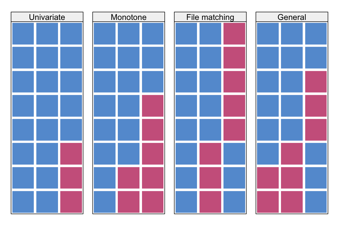
Figure 4.1: Some missing data patterns in multivariate data. Blue is observed, red is missing.

Figure 4.1 illustrates various data patterns in multivariate data. Monotone patterns can occur as a result of drop-out in longitudinal studies. If a pattern is monotone, the variables can be sorted conveniently according to the percentage of missing data. Univariate missing data form a special monotone pattern. Important computational savings are possible if the data are monotone.

All patterns displayed in Figure 4.1 are connected. The file matching pattern is connected since it is possible to travel to all blue cells by horizontal or vertical moves. This pattern will become unconnected if we remove the first column. In contrast, after removing the first column from the general pattern in Figure 4.1 it is still connected through the first two rows.

Connected patterns are needed to identify unknown parameters. For example, in order to be able to estimate a correlation coefficient between two variables, they need to be connected, either directly by a set of cases that have scores on both, or indirectly through their relation with a third set of connected data. Unconnected patterns may arise in particular data collection designs, like data combination of different variables and samples, or potential outcomes.

Missing data patterns of longitudinal data organized in the “long format” (cf. Section 11.1) are more complex than the patterns in Figure 4.1. See Van Buuren (2011, 179) for some examples.

4.1.2 Summary statistics

The missing data pattern influences the amount of information that can be transferred between variables. Imputation can be more precise if other variables are non-missing for those cases that are to be imputed. The reverse is also true. Predictors are potentially more powerful if they have are non-missing in rows that are vastly incomplete. This section discusses various measures of the missing data pattern.

The function md.pattern() in mice calculates the frequencies of the missing data patterns. For example, the frequency pattern of the dataset pattern4 in Figure 4.1 is

md.pattern(pattern4, plot = FALSE)

  A B C  
2 1 1 1 0
3 1 1 0 1
1 1 0 1 1
2 0 0 1 2
  2 3 3 8

The columns A, B and C are either 0 (missing) or 1 (observed). The first column provides the frequency of each pattern. The last column lists the number of missing entries per pattern. The bottom row provides the number of missing entries per variable, and the total number of missing cells. In practice, md.pattern() is primarily useful for datasets with a small number of columns.

Alternative measures start from pairs of variables. A pair of variables \((Y_j,Y_k)\) can have four missingness patterns:

1. both \(Y_j\) and \(Y_k\) are observed (patternrr);

2. \(Y_j\) is observed and \(Y_k\) is missing (pattern rm);

3. \(Y_j\) is missing and \(Y_k\) is observed (pattern mr);

4. both \(Y_j\) and \(Y_k\) are missing (pattern mm).

For example, for the monotone pattern in Figure 4.1 the frequencies are:

p <- md.pairs(pattern4)
p

$rr
  A B C
A 6 5 3
B 5 5 2
C 3 2 5

$rm
  A B C
A 0 1 3
B 0 0 3
C 2 3 0

$mr
  A B C
A 0 0 2
B 1 0 3
C 3 3 0

$mm
  A B C
A 2 2 0
B 2 3 0
C 0 0 3

Thus, for pair (A,B) there are five completely observed pairs (in rr), no pairs in which A is observed and B missing (in rm), one pair in which A is missing and B is observed (in mr) and two pairs with both missing A and B. Note that these numbers add up to the total sample size.

The proportion of usable cases (Van Buuren, Boshuizen, and Knook 1999) for imputing variable \(Y_j\) from variable \(Y_k\) is defined as

\[I_{jk} = \frac{\sum_i^n (1-r_{ij})r_{ik}}{\sum_i^n 1-r_{ij}} \]

This quantity can be interpreted as the number of pairs \((Y_j,Y_k)\) with \(Y_j\) missing and \(Y_k\) observed, divided by the total number of missing cases in \(Y_j\). The proportion of usable cases \(I_{jk}\) equals 1 if variable \(Y_k\) is observed in all records where \(Y_j\) is missing. The statistic can be used to quickly select potential predictors \(Y_k\) for imputing \(Y_j\) based on the missing data pattern. High values of \(I_{jk}\) are preferred. For example, we can calculate \(I_{jk}\) in the dataset pattern4 in Figure 4.1 for all pairs \((Y_j, Y_k)\) by

p$mr/(p$mr+p$mm)

      A B C
A 0.000 0 1
B 0.333 0 1
C 1.000 1 0

The first row contains \(I_{\mathrm{AA}}=0\), \(I_{\mathrm{AB}}=0\) and \(I_{\mathrm{AC}} = 1\). This informs us that B is not relevant for imputing A since there are no observed cases in B where A is missing. However, C is observed for both missing entries in A, and may thus be a relevant predictor. The \(I_{jk}\) statistic is an inbound statistic that measures how well the missing entries in variable \(Y_j\) are connected to the rest of the data.

The outbound statistic \(O_{jk}\) measures how observed data in variable \(Y_j\) connect to missing data in the rest of the data. The statistic is defined as

\[ O_{jk} = \frac{\sum_i^n r_{ij}(1-r_{ik})}{\sum_i^n r_{ij}} \]

This quantity is the number of observed pairs \((Y_j,Y_k)\) with \(Y_j\) observed and \(Y_k\) missing, divided by the total number of observed cases in \(Y_j\). The quantity \(O_{jk}\) equals 1 if variable \(Y_j\) is observed in all records where \(Y_k\) is missing. The statistic can be used to evaluate whether \(Y_j\) is a potential predictor for imputing \(Y_k\). We can calculate \(O_{jk}\) in the dataset pattern4 in Figure 4.1 for all pairs \((Y_j, Y_k)\) by

p$rm/(p$rm+p$rr)

    A     B   C
A 0.0 0.167 0.5
B 0.0 0.000 0.6
C 0.4 0.600 0.0

Thus A is potentially more useful to impute C (3 out of 6) than B (1 out of 6).

4.1.3 Influx and outflux

The inbound and outbound statistics in the previous section are defined for variable pairs \((Y_j,Y_k)\). This section describes two overall measures of how each variable connects to others: influx and outflux.

The influx coefficient \(I_j\) is defined as

\[ I_j = \frac{\sum_j^p\sum_k^p\sum_i^n (1-r_{ij})r_{ik}}{\sum_k^p\sum_i^n r_{ik}} \]

The coefficient is equal to the number of variable pairs \((Y_j,Y_k)\) with \(Y_j\) missing and \(Y_k\) observed, divided by the total number of observed data cells. The value of \(I_j\) depends on the proportion of missing data of the variable. Influx of a completely observed variable is equal to 0, whereas for completely missing variables we have \(I_j=1\). For two variables with the same proportion of missing data, the variable with higher influx is better connected to the observed data, and might thus be easier to impute.

The outflux coefficient \(O_j\) is defined in an analogous way as

\[ O_j = \frac{\sum_j^p\sum_k^p\sum_i^n r_{ij}(1-r_{ik})}{\sum_k^p\sum_i^n 1-r_{ij}} \]

The quantity \(O_j\) is the number of variable pairs with \(Y_j\) observed and \(Y_k\) missing, divided by the total number of incomplete data cells. Outflux is an indicator of the potential usefulness of \(Y_j\) for imputing other variables. Outflux depends on the proportion of missing data of the variable. Outflux of a completely observed variable is equal to 1, whereas outflux of a completely missing variable is equal to 0. For two variables having the same proportion of missing data, the variable with higher outflux is better connected to the missing data, and thus potentially more useful for imputing other variables.

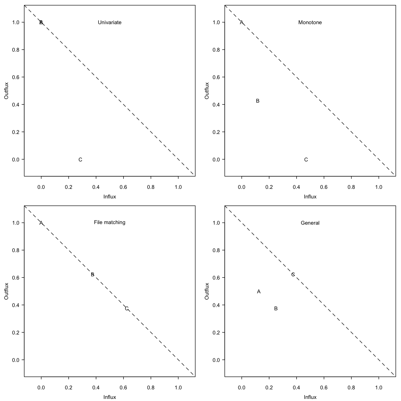
Figure 4.2: Outflux versus influx in the four missing data patterns from Figure 4.1. The influx of a variable quantifies how well its missing data connect to the observed data on other variables. The outflux of a variable quantifies how well its observed data connect to the missing data on other variables. In general, higher influx and outflux values are preferred.

The function flux() in mice calculates \(I_j\) and \(O_j\) for all variables. For example, for pattern4 we obtain

flux(pattern4)[,1:3]

   pobs influx outflux
A 0.750  0.125   0.500
B 0.625  0.250   0.375
C 0.625  0.375   0.625

The rows correspond to the variables. The columns contain the proportion of observed data, \(I_j\) and \(O_j\). Figure 4.2 shows the influx-outflux pattern of the four patterns in Figure 4.1 produced by fluxplot(). In general, variables that are located higher up in the display are more complete and thus potentially more useful for imputation. It is often (but not always) true that \(I_j+O_j\leq 1\), so in practice variables closer to the subdiagonal are typically better connected than those farther away. The fluxplot can be used to spot variables that clutter the imputation model. Variables that are located in the lower regions (especially near the lower-left corner) and that are uninteresting for later analysis are better removed from the data prior to imputation.

Influx and outflux are summaries of the missing data pattern intended to aid in the construction of imputation models. Keeping everything else constant, variables with high influx and outflux are preferred. Realize that outflux indicates the potential (and not actual) contribution to impute other variables. A variable with high \(O_j\) may turn out to be useless for imputation if it is unrelated to the incomplete variables. On the other hand, the usefulness of a highly predictive variable is severely limited by a low \(O_j\). More refined measures of usefulness are conceivable, e.g., multiplying \(O_j\) by the average proportion of explained variance. Also, we could specialize to one or a few key variables to impute. Alternatively, analogous measures for \(I_j\) could be useful. The further development of diagnostic summaries for the missing data pattern is a promising area for further investigation.