3.8 Nonignorable missing data
3.8.1 Overview
All methods described thus far assume that the missing data mechanism is ignorable. In this case, there is no need for an explicit model of the missing data process (cf. Section 2.2.6). In reality, the mechanism may be nonignorable, even after accounting for any measurable factors that govern the response probability. In such cases, we can try to adapt the imputed data to make them more realistic. Since such adaptations are based on unverifiable assumptions, it is recommended to study carefully the impact of different possibilities on the final inferences by means of sensitivity analysis.
When is the assumption of ignorability suspect? It is hard to provide cut-and-dried criteria, but the following list illustrates some typical situations:
If important variables that govern the missing data process are not available;
If there is reason to believe that responders differ from non-responders, even after accounting for the observed information;
If the data are truncated.
If ignorability does not hold, we need to model the distribution \(P(Y,R)\) instead of \(P(Y)\). For nonignorable missing data mechanisms, \(P(Y,R)\) do not factorize into independent parts. Two main strategies to decompose \(P(Y,R)\) are known as the selection model (Heckman 1976) and the pattern-mixture model (Glynn, Laird, and Rubin 1986). Little and Rubin (2002 ch. 15) and Little (2009) provide in-depth discussions of these models.
Imputations are created most easily under the pattern-mixture model. Herzog and Rubin (1983, 222–24) proposed a simple and general family of nonignorable models that accounts for shift bias, scale bias and shape bias. Suppose that we expect that the nonrespondent data are shifted relative to the respondent data. Adding a simple shift parameter \(\delta\) to the imputations creates a difference in the means of a \(\delta\). In a similar vein, if we suspect that the nonrespondents and respondents use different scales, we can multiply each imputation by a scale parameter. Likewise, if we suspect that the shapes of both distributions differ, we could redraw values from the candidate imputations with a probability proportional to the dissimilarity between the two distributions, a technique known as the SIR algorithm (Rubin 1987a). We only discuss the shift parameter \(\delta\).
In practice, it may be difficult to specify the distribution of the nonrespondents, e.g., to provide a sensible specification of \(\delta\). One approach is to compare the results under different values of \(\delta\) by sensitivity analysis. Though helpful, this puts the burden on the specification of realistic scenarios, i.e., a set of plausible \(\delta\)-values. The next sections describe the selection model and pattern mixture in more detail, as a way to evaluate the plausibility of \(\delta\).
3.8.2 Selection model
The selection model (Heckman 1976) decomposes the joint distribution \(P(Y,R)\) as
\[ P(Y,R) = P(Y)P(R|Y). \tag{3.8} \]
The selection model multiplies the marginal distribution \(P(Y)\) in the population with the response weights \(P(R|Y)\). Both \(P(Y)\) and \(P(R|Y)\) are unknown, and must be specified by the user. The model where \(P(Y)\) is normal and where \(P(R|Y)\) is a probit model is known as the Heckman model. This model is widely used in economics to correct for selection bias.
| \(Y\) | \(P(Y)\) | $P(R=1 | Y)$ | $P(Y |
|---|---|---|---|---|
| 100 | 0.02 | 0.65 | 0.015 | 0.058 |
| 110 | 0.03 | 0.70 | 0.024 | 0.074 |
| 120 | 0.05 | 0.75 | 0.043 | 0.103 |
| 130 | 0.10 | 0.80 | 0.091 | 0.164 |
| 140 | 0.15 | 0.85 | 0.145 | 0.185 |
| 150 | 0.30 | 0.90 | 0.307 | 0.247 |
| 160 | 0.15 | 0.92 | 0.157 | 0.099 |
| 170 | 0.10 | 0.94 | 0.107 | 0.049 |
| 180 | 0.05 | 0.96 | 0.055 | 0.016 |
| 190 | 0.03 | 0.98 | 0.033 | 0.005 |
| 200 | 0.02 | 1.00 | 0.023 | 0.000 |
| \(\bar Y\) | 150.00 | 151.58 | 138.60 |
Numerical example. The column labeled \(Y\) in Table 3.5 contains the midpoints of 11 categories of systolic blood pressure. The column \(P(Y)\) contains a hypothetically complete distribution of systolic blood pressure. It is specified here as symmetric with a mean of 150 mmHg (millimeters mercury). This distribution should be a realistic description of the combined observed and missing blood pressure values in the population of interest. The column \(P(R=1|Y)\) specifies the probability that blood pressure is actually observed at different levels of blood pressure. Thus, at a systolic blood pressure of 100 mmHg, we expect that 65% of the data will be observed. On the other hand, we expect that no missing data occur for those with a blood pressure of 200 mmHg. This specification produces 12.2% of missing data. The variability in the missingness probability is large, and reflects an extreme scenario where the missing data are created mostly at the lower blood pressures. Section 9.2.1 discusses why more missing data in the lower levels are plausible. When taken together, the columns \(P(Y)\) and \(P(R=1|Y)\) specify a selection model.
3.8.3 Pattern-mixture model
The pattern-mixture model (Glynn, Laird, and Rubin 1986; Little 1993) decomposes the joint distribution \(P(Y,R)\) as
\[\begin{align} P(Y,R)&=& P(Y|R)P(R) \tag{3.9}\\ &=& P(Y|R=1)P(R=1) + P(Y|R=0)P(R=0) \tag{3.10} \end{align}\]Compared to Equation (3.8) this model only reverses the roles of \(Y\) and \(R\), but the interpretation is quite different. The pattern-mixture model emphasizes that the combined distribution is a mix of the distributions of \(Y\) in the responders and nonresponders. The model needs a specification of the distribution \(P(Y|R=1)\) of the responders (which can be conveniently modeled after the data), and of the distribution \(P(Y|R=0)\) of the nonresponders (for which we have no data at all). The joint distribution is the mixture of these two distributions, with mixing probabilities \(P(R=1)\) and \(P(R=0)=1-P(R=1)\), the overall proportions of observed and missing data, respectively.
Numerical example. The columns labeled \(P(Y|R=1)\) and \(P(Y|R=0)\) in Table 3.5 contain the probability per blood pressure category for the respondents and nonrespondents. Since more missing data are expected to occur at lower blood pressures, the mass of the nonresponder distribution has shifted toward the lower end of the scale. As a result, the mean of the nonresponder distribution is equal to 138.6 mmHg, while the mean of the responder distribution equals 151.58 mmHg.
3.8.4 Converting selection and pattern-mixture models
The pattern-mixture model and the selection model are connected via Bayes rule. Suppose that we have a mixture model specified as the probability distributions \(P(Y|R=0)\) and \(P(Y|R=1)\) plus the overall response probability \(P(R)\). The corresponding selection model can be calculated as \[P(R=1|Y=y) = P(Y=y|R=1)P(R=1) / P(Y=y)\] where the marginal distribution of \(Y\) is
\[ P(Y=y) = P(Y=y|R=1)P(R=1) + P(Y=y|R=0)P(R=0) \tag{3.11} \]
Reversely, the pattern-mixture model can be calculated from the selection model as follows:
\[ P(Y=y|R=r) = P(R=r|Y=y)P(Y=y) / P(R=r) \tag{3.12} \]
where the overall probability of observed (\(r=1\)) or missing (\(r=0\)) data is equal to \[ P(R=r) = \sum_y P(R=r|Y=y)P(Y=y) (\#eq:overallprob) \]
Numerical example. In Table 3.5 we calculate \(P(Y=100) = 0.015 \times 0.878 + 0.058 \times 0.122 = 0.02\). Likewise, we find \(P(R=1|Y) = 0.015 \times 0.878 / 0.02 = 0.65\) and \(P(R=0|Y) = 0.058 \times 0.122/0.02 = 0.35\). The reverse calculation is left as an exercise to the reader.
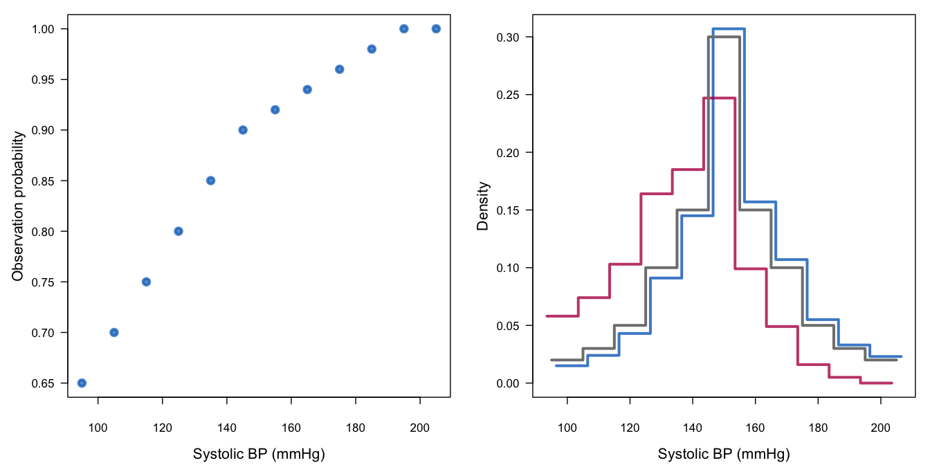
Figure 3.9: Graphic representation of the response mechanism for systolic blood pressure in Table 3.5. See text for explanation.
Figure 3.9 is an illustration of the posited missing data mechanism. The left-hand figure displays the missingness probabilities \(P(R|Y)\) of the selection model. The right-hand plot provides the distributions \(P(Y|R)\) in the observed (blue) and missing (red) data in the corresponding pattern-mixture model. The hypothetically complete distribution is given by the black curve. The distribution of blood pressure in the group with missing blood pressures is quite different, both in form and location. At the same time, observe that the effect of missingness on the combined distribution is only slight. The reason is that 87% of the information is actually observed.
The mean of the distribution of the observed data remains almost unchanged (151.6 mmHg instead of 150 mmHg), but the mean of the distribution of the missing data is substantially lower at 138.6 mmHg. Thus, under the assumed selection model we expect that the mean of the imputed data should be \(151.6-138.6 = 13\) mmHg lower than in the observed data.
3.8.5 Sensitivity analysis
Sections 3.8.2–3.8.4 provide different, though related, views on the assumed response model. A fairly extreme response model where the missingness probability increases from 0% to 35% in the outcome produces a mean difference of 13 mmHg. The effect in the combined distribution is much smaller: 1.6 mmHg.
| \(\delta\) | Interpretation | |
|---|---|---|
| \(0\) mmHg | MCAR, \(\delta\) too small | |
| \(-5\) mmHg | Small effect | |
| \(-10\) mmHg | Large effect | |
| \(-15\) mmHg | Extreme effect | |
| \(-20\) mmHg | Too extreme effect |
Section 3.8.1 discussed the idea of adding some extra mmHg to the imputed values, a method known as \(\delta\)-adjustment. It is important to form an idea of what reasonable values for \(\delta\) could be. Under the posited model, \(\delta=0\) mmHg is clearly too small (as it assumes MCAR), whereas \(\delta=-20\) mmHg is too extreme (as it can only occur if nearly all missing values occur in the lowest blood pressures). Table 3.6 provides an interpretation of various values for \(\delta\). The most likely scenarios would yield \(\delta=-5\) or \(\delta=-10\) mmHg.
In practice, part of \(\delta\) may be realized through the predictors needed under MAR. It is useful to decompose \(\delta\) as \(\delta = \delta_\mathrm{MAR} + \delta_\mathrm{MNAR}\), where \(\delta_\mathrm{MAR}\) is the mean difference caused by the predictors in the imputation models, and where \(\delta_\mathrm{MNAR}\) is the mean difference caused by an additional nonignorable part of the imputation model. If candidate imputations are produced under MAR, we only need to add a constant \(\delta_\mathrm{MNAR}\). Section 9.2 continues this application.
Adding a constant may seem overly simple, but it is actually quite powerful. In cases where no one model will be obviously more realistic than any other, Rubin (1987b, 203) stressed the need for easily communicated models, like a “20% increase over the ignorable value.” Little (2009, 49) warned that it is easy to be enamored of complicated models for \(P(Y,R)\) so that we may be “lulled into a false sense of complacency about the fundamental lack of identification,” and suggested simple methods:
The idea of adding offsets is simple, transparent, and can be readily accomplished with existing software.
Adding a constant or multiplying by a value are in fact the most direct ways to specify nonignorable models.
3.8.6 Role of sensitivity analysis
Nonignorable models are only useful after the possibilities to make the data “more MAR” have been exhausted. A first step is always to create the best possible imputation model based on the available data. Section 6.3.2 provides specific advice on how to build imputation models.
The MAR assumption has been proven defensible for intentional missing data. In general, however, we can never rule out the possibility that the data are MNAR. In order to cater for this possibility, many advise performing a sensitivity analysis on the final result. This is voiced most clearly in recommendation 15 of the National Research Council’s advice on clinical trials (National Research Council 2010):
Recommendation 15: Sensitivity analysis should be part of the primary reporting of findings from clinical trials. Examining sensitivity to the assumptions about the missing data mechanism should be a mandatory component of reporting.
While there is much to commend this rule, we should refrain from doing sensitivity analysis just for the sake of it. The proper execution of a sensitivity analysis requires us to specify plausible scenarios. An extreme scenario like “suppose that all persons who leave the study die” can have a major impact on the study result, yet it could be highly improbable and therefore of limited interest.
Sensitivity analysis on factors that are already part of the imputation model is superfluous. Preferably, before embarking on a sensitivity analysis, there should be reasonable evidence that the MAR assumption is (still) inadequate after the available data have been taken into account. Such evidence is also crucial in formulating plausible MNAR mechanisms. Any decisions about scenarios for sensitivity analysis should be taken in discussion with subject-matter specialists. There is no purely statistical solution to the problem of nonignorable missing data. Sensitivity analysis can increase our insight into the stability of the results, but in my opinion we should only use it if we have a firm idea of which scenarios for the missingness would be reasonable.
In practice, we may lack such insights. In such instances, I would prefer a carefully constructed imputation model (which is based on all available data) over a poorly constructed sensitivity analysis.
3.8.7 Recent developments
The literature on nonignorable models is large and diverse. The research in this area is active and recent. This section provides some pointers into the recent literature.
The historic overview by Kenward and Molenberghs (2015) provides an in-depth treatment of the selection, pattern-mixture and shared parameter models, including their connnections. The Handbook of Missing Data Methodology (Molenberghs et al. 2015) contains five chapters that discuss sensitivity analysis from all angles. The handbook should be the starting point for anyone considering models for data that are MNAR. Little, Rubin, and Zangeneh (2017) developed an alternative strategy based on selecting a subset of parameters of substantive interest. In particular cases, the conditions for ignoring the missing-data mechanism are more relaxed than under MAR.
Regulators prefer simple methods that impute the missing outcomes under MAR, and then add an adjustment \(\delta\) to the imputes, while varying \(\delta\) over a plausible range and independently for each treatment group (Permutt 2016). The most interesting scenarios will be those where the difference between the \(\delta\)’s correspond to the size of the treatment effect in the completers. Contours of the \(p\)-values may be plotted on a graph as a function of the \(\delta\)’s to assist in a tipping-point analysis (Liublinska and Rubin 2014).
Kaciroti and Raghunathan (2014) relate the identifying parameters from the pattern-mixture model to the corresponding missing data mechanism in the selection model. This dual interpretation provides a unified framework for performing sensitivity analysis. Galimard et al. (2016) proposed an imputation method under MNAR based on the Heckman model. The random indicator method (Jolani 2012) is an experimental iterative method that redraws the missing data indicator under a selection model, and imputes the missing data under a pattern-mixture model, with the objective of estimating \(\delta\) from the data under relaxed assumptions. Initial simulation results look promising. The algorithm is available as the ri method in mice.